Stacked Generalization Machine Learning: Advanced Predictive Modeling for Material Stability and Drug Development

Abstract

This article provides a comprehensive exploration of stacked generalization, an advanced ensemble machine learning technique, and its application in predicting material stability and properties crucial for drug development. It covers foundational concepts, methodological implementation, optimization strategies, and comparative validation. Tailored for researchers and pharmaceutical professionals, the content demonstrates how stacking integrates multiple base models with a meta-learner to achieve superior predictive accuracy and robustness compared to single-model approaches. By incorporating real-world case studies and interpretability frameworks like SHAP, this guide serves as a practical resource for developing reliable predictive models that can accelerate material discovery and formulation in biomedical research.

Stacked Generalization Fundamentals: From Core Concepts to Material Science Applications

Stacked generalization, commonly known as stacking, represents an advanced ensemble machine learning method that integrates multiple predictive models through a meta-learning framework to achieve superior performance compared to any single constituent model. This approach systematically deduces and corrects the biases of base learners by combining their predictions in an optimally weighted manner, typically through cross-validation and a meta-learner architecture. First introduced by Wolpert in 1992, stacked generalization has evolved into formal implementations like the Super Learner, with proven theoretical guarantees that it performs asymptotically at least as well as the best individual model in the ensemble [1] [2]. While initially conceptualized decades ago, stacking has gained significant traction in recent years across diverse fields including genomic selection, energy systems prognostics, and medical diagnostics, demonstrating its capacity to enhance predictive accuracy, improve robustness, and mitigate overfitting [3] [4] [5]. This protocol outlines the fundamental principles, implementation workflows, and practical applications of stacked generalization, providing researchers with a structured framework for deploying this advanced ensemble method in computational research, particularly in material stability and drug development contexts.

Conceptual Foundation and Historical Development

Stacked generalization operates on the principle of combining multiple "level-zero" base algorithms through a "higher-level" meta-model that learns how to optimally integrate their predictions [1]. Unlike simpler ensemble methods like bagging or boosting that typically combine homogeneous model types through averaging or weighted voting, stacking leverages heterogeneous models that capture different aspects of the underlying patterns in the data [6]. The meta-model in stacking effectively learns the relative competencies of each base learner across different regions of the feature space, creating a sophisticated combination that capitalizes on their collective strengths while mitigating individual weaknesses.

The methodology was first formally introduced by David Wolpert in 1992 as a scheme for minimizing generalization error by deducing the biases of generalizers with respect to a provided learning set [2]. Wolpert demonstrated that stacked generalization could be viewed as a more sophisticated version of cross-validation, employing strategies beyond simple winner-takes-all combinations. Later developments by Breiman and van der Laan et al. established theoretical foundations, including constraints for convex combinations and proofs of asymptotic optimality [1] [3]. The formalization of the Super Learner algorithm by van der Laan and colleagues provided a rigorous implementation framework with V-fold cross-validation at its core, establishing stacking as a theoretically grounded approach with guaranteed performance properties [1].

Theoretical Advantages and Performance Guarantees

The principal theoretical advantage of stacked generalization lies in its asymptotic performance guarantee – in large samples, the algorithm will perform at least as well as the best individual predictor included in the ensemble [1]. This property makes stacking particularly valuable in research contexts where model selection uncertainty exists, as it provides insurance against selecting a suboptimal single model. The diversity of the base learner library is crucial to this performance; a larger and more diverse library enhances the potential for superior performance [1].

Stacking demonstrates particular effectiveness in addressing the bias-variance tradeoff inherent in predictive modeling. By combining multiple models with different inductive biases, stacking reduces both variance (through averaging effects) and bias (through complementary model strengths) [6]. Furthermore, the cross-validation framework inherent in proper stacking implementation provides robust protection against overfitting, as the meta-learner is trained on out-of-sample predictions from the base models [1] [7]. This makes stacking particularly valuable for small to moderate-sized datasets common in scientific research, where overfitting presents a significant concern.

Fundamental Principles and Methodology

Core Architecture and Components

The architecture of stacked generalization consists of two primary layers: the base model layer (level-zero models) and the meta-model layer (level-one learner) [4]. The base models comprise a diverse collection of prediction algorithms, which can include parametric regression models, non-parametric methods, and complex machine learning approaches. These models are chosen specifically for their complementary strengths and diverse inductive biases. The meta-model is a learning algorithm that takes the predictions from the base models as its input features and learns to combine them optimally to produce the final prediction [3] [4].

The combination process in stacking is typically implemented under specific constraints to ensure stability and performance. Commonly, a convex combination is enforced, requiring non-negative weights that sum to one [1]. This constraint improves numerical stability and interpretability while maintaining theoretical performance guarantees. The objective function for this combination is typically aligned with the research goal, such as minimizing mean squared error for continuous outcomes or maximizing area under the ROC curve for classification tasks [1].

The Cross-Validation Foundation

A critical methodological component of stacked generalization is the use of V-fold cross-validation to generate inputs for the meta-model [1] [7]. This process involves:

• Splitting the training data into V mutually exclusive and exhaustive folds
• For each fold v, training each base model on all data except fold v
• Using these trained models to generate predictions for the held-out fold v
• Collecting these cross-validated predictions for all observations to create a new dataset (the "level-one" data) where each instance contains the base model predictions and the true outcome value [1]

This cross-validation framework ensures that the predictions used to train the meta-model are truly out-of-sample for each base model, preventing information leakage and overfitting. The resulting level-one data has the same size as the original training set but contains the base models' generalized predictions rather than the original features [7].

The following diagram illustrates the complete stacked generalization workflow, from initial data partitioning to final model generation:

Implementation Protocols

Standard Super Learner Protocol

The following step-by-step protocol implements the standard Super Learner, which represents a formalized implementation of stacked generalization:

Table 1: Step-by-Step Super Learner Protocol

Step	Action	Key Considerations
1. Data Partitioning	Split data into V mutually exclusive folds (typically V=5 or V=10)	Ensure folds maintain distribution of outcome; stratify for classification
2. Base Model Training	For each fold v, train each base model on all data except fold v	Use diverse algorithms (GAM, splines, random forests, etc.) [1]
3. Cross-validation Prediction	Use each trained base model to predict outcomes for held-out fold v	Store these out-of-sample predictions for all observations
4. Risk Estimation	For each algorithm, compute average performance across all folds	Use appropriate loss function (MSE for continuous, rank loss for AUC) [1]
5. Level-One Data Creation	Create new dataset with CV predictions as features and true outcomes as response	This dataset has same number of rows as original training data
6. Meta-Learner Training	Train meta-model on level-one data to combine base model predictions	Use non-negative least squares or constrained regression [1]
7. Full Model Training	Retrain all base models on complete training dataset	Maintains maximum information for final predictions
8. Prediction Generation	Combine full base model predictions using meta-learner weights	Apply to new data using the complete stacked system

This protocol emphasizes the critical distinction between the cross-validation phase (steps 2-4) used to generate training data for the meta-learner, and the final model building phase (steps 7-8) that utilizes the entire dataset for maximum predictive performance [1]. The risk estimation in step 4 provides a honest assessment of each base model's performance and can be used for the Discrete Super Learner (selecting the single best model) even if proceeding to full stacking.

Advanced Implementation: Evolutionary Stacked Generalization

For complex prediction problems with high-dimensional feature spaces, such as those encountered in material stability research or genomic selection, an evolutionary optimization approach can enhance standard stacking:

Table 2: Evolutionary Stacking Enhancement Protocol

Component	Standard Approach	Evolutionary Enhancement
Feature Selection	Use all available features or manual selection	Implement MIC and AIC for automated input variable selection [4]
Hyperparameter Tuning	Manual tuning or grid search	Apply improved Grasshopper Optimization Algorithm (IGOA) [4]
Base Model Selection	Pre-specified model types	Algorithmic selection of complementary models with low correlation [4]
Meta-Learner Training	Standard regression or classification	Regularized Extreme Learning Machine (RELM) for enhanced generalization [4]
Validation	Standard V-fold cross-validation	Nested cross-validation with optimization in inner loops

The evolutionary approach introduces intelligent optimization at multiple stages of the stacking pipeline, addressing key challenges in complex domains. The Maximum Information Coefficient (MIC) and Akaike Information Criterion (AIC) component selects input variables by measuring correlation between features and outputs, reducing dimensionality while retaining predictive information [4]. The Improved Grasshopper Optimization Algorithm (IGOA) enhances hyperparameter tuning through Chebyshev chaotic mapping initialization and spiral position update mechanisms, avoiding local optima while searching for optimal model configurations [4].

Application Case Studies Across Domains

Genomic Selection in Plant and Animal Breeding

Stacked generalization has demonstrated significant value in genomic selection, where the goal is to predict breeding values for desirable traits based on genome-wide markers:

Table 3: Stacking Performance in Genomic Selection Applications

Species	Dataset Characteristics	Base Models	Performance Results
Rice	3,686 SNPs from 198 accessions, 30 quantitative traits [3]	Six linear mixed and Bayesian models [3]	Lower or comparable MSE to individual methods; reduced overfitting [3]
Barley	5,160 SNPs from 307 accessions, 8 traits [3]	rrBLUP, gBLUP, Bayesian models [3]	Superior stability across different trait types [3]
Maize	45,438 SNPs from 262 accessions, 11 traits [3]	Linear mixed models and nonlinear alternatives [3]	Consistent performance across environmental conditions [3]
Mice	10,346 SNPs from 1,181 samples, 20 traits [3]	Bayesian and mixed effect models [3]	Resistance to overfitting demonstrated through hypothesis testing [3]

In these genomic selection applications, stacking integrated methods including rrBLUP (ridge regression BLUP), gBLUP (genomic BLUP), and various Bayesian models (BayesA, BayesB) [3]. The meta-model employed was typically a neural network (multi-layer perceptron) that learned to weight the contributions of each base model according to their predictive strengths for specific traits [3]. This approach proved particularly valuable given that no single method demonstrated universal superiority across all traits, species, and environmental conditions, echoing the fundamental premise that stacking performance depends on library diversity [3].

Energy Systems Prognostics

In prognostics and health management for energy systems, stacking has addressed the challenging problem of predicting remaining useful life (RUL) of proton exchange membrane fuel cells (PEMFC):

This architecture combines support vector regression (SVR) for its high-dimensional data processing capabilities with gated recurrent units (GRU) for their strong sequence learning capacity [4]. The meta-model employs a regularized extreme learning machine (RELM) that provides stable generalization ability [4]. Experimental results demonstrated that this stacked approach outperformed individual models across different operating conditions, achieving superior prediction accuracy for future degradation trend and remaining useful life [4].

Medical Diagnostics and Cancer Detection

Stacked generalization has shown remarkable performance in medical diagnostics, particularly in cancer detection where accurate classification is critical:

Table 4: Stacking for Cancer Detection Performance

Dataset	Characteristics	Base Models	Meta-Model	Performance
WBC (Breast Cancer)	569 patients, 30 features, 37.2% malignant cases [5]	Logistic Regression, Naïve Bayes, Decision Tree [5]	Multilayer Perceptron [5]	100% accuracy with 6 selected features [5]
LCP (Lung Cancer)	15 features, binary classification [5]	Logistic Regression, Naïve Bayes, Decision Tree [5]	Multilayer Perceptron [5]	100% accuracy with 5 selected features [5]

The cancer detection application employed a sophisticated multistage feature selection process combining filter, wrapper, and embedded methods to reduce the feature space while maintaining diagnostic information [5]. The stacking ensemble leveraged the complementary strengths of logistic regression (linear relationships), Naïve Bayes (probabilistic structure), and decision trees (nonlinear interactions) [5]. The multilayer perceptron meta-model learned to optimally combine these diverse perspectives, achieving perfect classification performance on benchmark datasets with reduced feature sets [5]. This demonstrates stacking's capacity to integrate multiple modeling paradigms while maintaining interpretability through feature selection.

Research Reagent Solutions

Implementing effective stacked generalization requires both computational frameworks and methodological components. The following table details essential "research reagents" for constructing stacked models:

Table 5: Essential Research Reagents for Stacked Generalization

Reagent Category	Specific Examples	Function/Purpose	Implementation Considerations
Base Model Algorithms	Generalized additive models (GAM) with splines [1]; Multivariate adaptive regression splines (MARS/earth) [1]; Bayesian GLMs [1]; Polynomial adaptive regression splines [1]; Support vector regression [4]; Gated recurrent units [4]	Capture diverse patterns and relationships in data	Select for complementarity rather than individual performance [4]
Meta-Learners	Non-negative least squares [1]; Regularized extreme learning machine [4]; Multilayer perceptron [5]; Logistic regression [3]	Optimally combine base model predictions	Constrain to convex combinations for stability [1]
Optimization Tools	Improved grasshopper optimization algorithm (IGOA) [4]; V-fold cross-validation [1]; Maximum information coefficient [4]	Tune hyperparameters and select features	Implement chaotic decreasing factors to avoid local optima [4]
Feature Selection Methods	Maximum information coefficient (MIC) [4]; Akaike information criterion (AIC) [4]; Hybrid filter-wrapper approaches [5]	Identify informative feature subsets	Balance relevance with redundancy reduction [5]
Validation Frameworks	5-fold or 10-fold cross-validation [1]; Nested cross-validation; Statistical hypothesis testing [3]	Provide honest performance assessment and prevent overfitting	Ensure computational feasibility with complex ensembles

These research reagents constitute the essential methodological toolkit for implementing stacked generalization across diverse domains. The selection of base models should prioritize architectural diversity and complementary inductive biases rather than simply choosing the best-performing individual models [4]. Similarly, meta-learners should be matched to the characteristics of the prediction task, with regularization employed to maintain generalization performance [1] [4]. The optimization and validation components ensure that the stacked ensemble achieves its theoretical performance advantages in practical applications.

Stacked generalization represents a sophisticated ensemble methodology that transcends simple model averaging or voting schemes by implementing a principled, meta-learning approach to combination. Through its cross-validation foundation and theoretical performance guarantees, stacking provides researchers with a robust framework for maximizing predictive accuracy while mitigating overfitting. The protocol outlined in this document provides both standard and advanced implementations suitable for various research contexts, from genomic selection to energy prognostics and medical diagnostics.

The case studies demonstrate stacking's versatility across domains with distinct data characteristics and modeling challenges. In genomic selection, stacking integrated diverse linear and Bayesian models to achieve stable performance across species and traits [3]. In energy systems, it combined temporal and structural models for accurate remaining useful life prediction [4]. In medical diagnostics, stacking with feature selection achieved perfect classification while maintaining interpretability [5]. These successes highlight stacking's capacity to synthesize diverse modeling perspectives into superior predictive performance.

For researchers pursuing material stability studies or drug development applications, stacked generalization offers a powerful approach to navigating model uncertainty and complexity. By implementing the protocols and leveraging the reagent solutions described herein, scientists can build ensembles that adapt to their specific data environments and research questions, ultimately accelerating discovery through enhanced predictive capability.

Stacked generalization, or stacking, is an advanced ensemble machine learning technique designed to enhance predictive performance by combining multiple models. Unlike bagging or boosting, which aggregate homogeneous models, stacking integrates diverse, or heterogeneous, models through a layered learning architecture [8] [9]. This approach is particularly powerful in complex research domains such as material stability and drug development, where it leverages the strengths of various algorithms to achieve superior accuracy and generalization [10] [11]. This article details the core architecture of stacking—encompassing base learners, meta-learners, and the operational workflow—framed within the context of computational material science research.

Core Concepts of Stacked Generalization

The architecture of stacking is structured into two primary layers: the base layer and the meta-layer.

• Base Learners (Level-0 Models): This layer consists of multiple, diverse machine learning models that are trained directly on the original dataset [9]. The strength of stacking relies on this diversity; using different algorithms (e.g., Decision Trees, Support Vector Machines, and linear models) ensures that each model captures unique patterns and relationships within the data [8]. The predictions of these models form the basis for the next layer of learning.

• Meta-Learner (Level-1 Model): The meta-learner is a model that learns how to best combine the predictions made by the base learners [8] [9]. Instead of being trained on the original features, it is trained on a new dataset composed of the cross-validated predictions from the base models. Its purpose is to discern when each base model is most reliable and to integrate their outputs optimally for a final prediction [8].

The "Super Learner" algorithm, a formalization of stacking, provides a theoretical guarantee that the stacked ensemble will perform as well as or better than any single base model included in the ensemble, asymptotically [8].

The Stacking Workflow: A Detailed Protocol

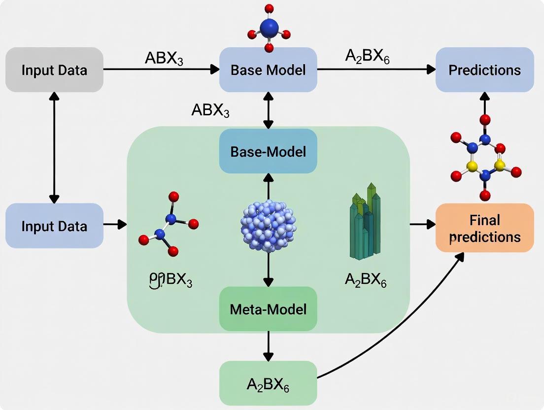
The process of building a stacked ensemble requires a systematic, multi-stage workflow to prevent data leakage and ensure robust generalization. The following protocol, illustrated in Figure 1, outlines these critical steps.

Figure 1. Stacked Generalization Workflow. This diagram illustrates the two-stage training process involving base learners and a meta-learner, using k-fold cross-validation to prevent overfitting.

Protocol 1: Construction of the Stacked Ensemble

This protocol describes the end-to-end process for creating a stacked model, from data partitioning to final model generation [8] [9].

• Step 1: Data Preparation and Partitioning. Split the full dataset into a training set and a hold-out test set. The training set will be used for all model development and validation, while the test set will be reserved for the final evaluation of the stacked ensemble.
• Step 2: Base Learner Training with k-Fold Cross-Validation. For each base learner, train the model using k-fold cross-validation on the training set.
  • Use the same k-fold splits for every base learner to ensure consistency [8].
  • For each fold, train the model on (k-1) folds and generate predictions on the withheld validation fold.
  • Collect these out-of-fold predictions for each data point in the training set. These are known as the cross-validated predictions.
• Step 3: Create the Level-One Data Matrix. Combine the cross-validated predictions from all base learners into a new feature matrix, often denoted as Z. Each column in Z represents the predictions from one base learner, and each row corresponds to a data point in the original training set. The true target values (y) for the training set are retained as the labels for this new matrix.
• Step 4: Train the Meta-Learner. Train the chosen meta-learning algorithm on the level-one data matrix (Z) and the true target values. The meta-learner learns the optimal way to weight and combine the predictions of the base learners.
• Step 5: Refit Base Learners and Finalize Ensemble. Retrain each of the base learners on the entire, original training set (without cross-validation). The final stacked ensemble consists of these fully-trained base learners and the trained meta-learner.

Protocol 2: Generating Predictions with the Stacked Ensemble

This protocol outlines the procedure for using the trained stacked ensemble to make predictions on new, unseen data [9].

• Step 1: Generate Base-Level Predictions. Pass the new data instance through each of the trained base learners to obtain a set of initial predictions.
• Step 2: Create Level-One Instance. Collect the predictions from all base learners for this instance and form them into a new feature vector, which is a single row with the same structure as the level-one data matrix Z.
• Step 3: Generate Final Prediction. Feed this new feature vector into the trained meta-learner, which will produce the final, ensemble prediction.

Performance Metrics and Quantitative Comparison

The effectiveness of a stacked ensemble is validated through rigorous comparison against its constituent models. The following table summarizes typical performance metrics from a materials informatics study predicting the work function of MXenes, where a stacked model achieved state-of-the-art results [10].

Table 1: Comparative Performance of Stacked Model vs. Base Learners in MXene Work Function Prediction

Model / Metric	Coefficient of Determination (R²)	Mean Absolute Error (MAE)	Root Mean Square Error (RMSE)
Stacked Model	0.95	0.20	N/A
Base Learner A	0.89	0.28	N/A
Base Learner B	0.91	0.25	N/A
Base Learner C	0.87	0.30	N/A

Note: Data adapted from a study on predicting MXenes' work function using stacked machine learning [10].

The superior performance of the stacked ensemble, as evidenced by the higher R² and lower MAE, highlights its capacity to integrate the strengths of individual models and mitigate their weaknesses. This leads to more accurate and robust predictions, which is critical in research applications.

Essential Research Reagents and Computational Tools

Implementing a stacked ensemble requires a suite of software libraries and computational tools. The table below functions as a "Scientist's Toolkit," detailing key "research reagents" for a successful stacking experiment.

Table 2: Research Reagent Solutions for Stacking Experiments

Reagent / Tool Name	Type / Category	Primary Function in Stacking Protocol
Scikit-learn	Python Library	Provides a unified API for implementing base learners (e.g., RF, SVM) and meta-learners, as well as tools for data preprocessing and k-fold cross-validation [10].
H2O.ai	AutoML Platform	Offers an automated and highly scalable implementation for training and tuning stacked ensembles, including built-in cross-validation management [8] [11].
MLxtend	Python Library	Contains a user-friendly StackingClassifier and StackingRegressor that simplifies the process of building stacked models without manual level-one data creation [9].
Pandas	Python Library	Essential for data manipulation, feature engineering, and the construction of the level-one data matrix from cross-validated predictions [10] [9].
SHAP	Interpretation Tool	Explains the output of the stacked ensemble by quantifying the contribution of each base learner's prediction to the final meta-learner's output, enhancing interpretability [10] [11].

Advanced Architectural Considerations

For researchers aiming to optimize a stacked ensemble, several advanced considerations are critical.

• Base Learner Diversity: The greatest gains from stacking are realized when the base learners are highly variable and make uncorrelated errors [8]. Combining a diverse set of algorithms (e.g., tree-based models, linear models, kernel-based models) is more effective than using multiple instances of the same algorithm type.
• Meta-Learner Selection: While any algorithm can serve as the meta-learner, simpler models are often preferred. Regularized linear models (e.g., LASSO or Ridge Regression) are common choices as they help prevent overfitting by assigning weights to the base learners' predictions. Random Forests or Gradient Boosting Machines can also be effective, particularly for capturing non-linear combinations [8].
• Mitigating Overfitting: The use of k-fold cross-validated predictions to build the level-one data matrix is the primary defense against overfitting [8]. This ensures that the meta-learner is trained on predictions that the base models made on data they were not directly trained on. An additional measure is to use a hold-out set, distinct from the training set used for base learner CV, to train the meta-learner.
• Interpretability with SHAP: The "black box" nature of complex ensembles can be mitigated using SHapley Additive exPlanations (SHAP). SHAP values can be applied to the meta-learner to interpret its behavior, showing how much each base model's prediction pushed the final output higher or lower for a given instance, thus providing global and local interpretability [10] [11].

The architectural relationship between data, base learners, and the meta-learner in a functioning stacked ensemble is summarized in the following system diagram.

Figure 2. Stacking Ensemble Inference Architecture. This diagram shows the data flow when a new instance is processed by the trained ensemble to produce a final prediction.

Stacked generalization, commonly known as stacking, is an advanced ensemble machine learning method that combines multiple base models through a meta-learning framework to enhance predictive performance and generalization capabilities. Unlike conventional ensemble approaches that use simple averaging or voting, stacking employs a learned combination mechanism where predictions from diverse base models serve as input features for a meta-model that generates final predictions. This architecture enables the ensemble to capitalize on the unique strengths of individual algorithms while mitigating their weaknesses, typically reducing prediction variance and improving robustness on unseen data.

In materials science research, particularly in stability prediction and property optimization, stacking has demonstrated remarkable effectiveness in addressing complex nonlinear relationships between composition, processing parameters, and material performance. Recent applications across diverse domains—from predicting MXenes' work functions to forecasting hardness in high-entropy nitride coatings and assessing dump slope stability in geotechnical engineering—consistently show that stacked ensembles outperform individual models, achieving performance improvements of approximately 10% or higher in multiple studies [10] [11] [12]. The method's ability to manage high-dimensional data with complex interactions makes it particularly valuable for materials informatics where traditional trial-and-error approaches are computationally prohibitive.

Theoretical Foundations: Variance Reduction Mechanisms

The Bias-Variance Decomposition Framework

The theoretical superiority of stacking originates from its nuanced approach to the bias-variance tradeoff, fundamental to supervised learning. A model's expected prediction error can be decomposed into three components: bias (error from erroneous assumptions), variance (error from sensitivity to fluctuations in training data), and irreducible error. Single complex models often achieve low bias but high variance, making them prone to overfitting. Stacking addresses this limitation through two primary mechanisms:

Diversity Integration: By combining multiple algorithms with different inductive biases (e.g., tree-based methods, linear models, support vector machines), stacking creates an ensemble where individual models make uncorrelated errors. When these diverse predictions are optimally combined, errors tend to cancel out, significantly reducing overall variance without substantially increasing bias [13] [8].

Meta-Learning Optimization: The meta-model learns optimal weighting schemes for base model predictions, effectively functioning as a adaptive bias-variance balancer. Theoretical work has established that super learners represent an asymptotically optimal system for learning, guaranteed to perform at least as well as the best single base model in large samples [1] [8].

Mathematical Formalization of Stacking

The stacking framework can be formally described as a two-level learning process. Given a set of L base models ( M1, M2, ..., ML ) and a dataset ( D = {(xi, yi)}{i=1}^N ), the first level generates cross-validated predictions from each base model. These predictions form a new feature matrix ( Z ) where each column ( Zj ) contains predictions from model ( Mj ). The meta-model then learns the mapping:

[ f_{\text{meta}}: Z \rightarrow Y ]

This secondary learning process enables the ensemble to identify contexts where specific base models excel, creating a specialized delegation system that no single model can achieve independently [1] [8]. The convex combination constraint often applied to meta-learning weights (( \alphak \geq 0, \sum{k=1}^L \alpha_k = 1 )) further enhances stability by preventing extreme weight assignments [1].

Quantitative Performance Evidence Across Domains

Recent empirical studies across multiple scientific domains provide compelling evidence of stacking's effectiveness for improving generalization. The following table summarizes key performance comparisons between stacked ensembles and individual models:

Table 1: Performance Comparison of Stacked Models vs. Individual Algorithms

Application Domain	Best Individual Model Performance (R²)	Stacked Model Performance (R²)	Performance Improvement	Key Metrics
MXenes Work Function Prediction [10]	0.85-0.90 (estimated)	0.95	~10%	MAE: 0.2 eV
Refractory HEN Coating Hardness [12]	~0.82	0.901	10%	-
Dump Slope Stability Prediction [11]	Varies by algorithm	H2O AutoML best performer	Outperformed all base models	R², MAE, RMSE
Boston Housing Price Prediction [8]	Varies by algorithm	Superior to individual models	Optimal combination	RMSE reduction

The consistency of these improvements across different domains and data characteristics underscores stacking's robustness. Particularly notable is the MXenes study, where stacking achieved a remarkably low mean absolute error of 0.2 eV while maintaining high interpretability through SHAP analysis [10]. In the refractory metal high-entropy nitride coatings research, the 10% accuracy improvement translated to practically significant gains in predicting mechanical properties under extreme conditions [12].

Table 2: Error Metric Comparisons Across Stacking Applications

Study	Base Model MAE/RMSE	Stacked Model MAE/RMSE	Variance Reduction
MXenes Work Function [10]	~0.26 eV (literature)	0.2 eV	23% improvement
Dump Slope Stability [11]	Varies by model	H2O AutoML minimal	Significant variance reduction
Super Learner Demonstration [1]	GAM: 2.58, Earth: 2.48 (MSE)	0.387×GAM + 0.613×Earth	Optimal weighted combination

Beyond accuracy metrics, stacking demonstrates superior stability in creation—the consistency of model outputs when trained with different random seeds or environmental variations. While individual models like random forests and deep neural networks can exhibit significant output variations based on initialization parameters, stacked ensembles show greater stability, particularly when base model diversity is properly managed [14].

Implementation Protocols for Materials Research

Standardized Stacking Workflow

The following experimental protocol outlines a systematic approach for implementing stacked generalization in materials stability research:

Phase 1: Data Preparation and Feature Engineering

• Curate high-quality datasets with comprehensive feature representation, including composition descriptors, processing parameters, and stability metrics
• Implement rigorous data cleaning procedures addressing missing values using appropriate imputation methods (Random Forest imputation demonstrated superior performance in HEN coatings study [12])
• Conduct feature selection to reduce dimensionality while preserving physical significance (e.g., using Pearson correlation thresholds |R| = 0.85 for feature grouping as in MXenes research [10])
• Partition data into training (80%), validation (10%), and test sets (10%) with stratification to maintain distribution consistency

Phase 2: Base Model Selection and Training

• Select diverse, high-performance algorithms spanning different learning paradigms (e.g., Random Forests, Gradient Boosting Machines, XGBoost, Support Vector Regressors, Neural Networks)
• Implement k-fold cross-validation (typically V=5 or V=10) with identical fold assignments across all base models to ensure consistent comparison
• Train each base model on the training set while preserving cross-validated predictions using settings like keep_cross_validation_predictions = TRUE in h2o [8]
• Perform hyperparameter optimization for each base model using Bayesian optimization or grid search

Phase 3: Meta-Model Development

• Construct level-one data by combining cross-validated predictions from all base models into an N×L feature matrix, where N is training sample size and L is number of base models
• Select an appropriate meta-learning algorithm (linear models, regularized regression, and random forests are common choices)
• Train the meta-model on level-one data to learn optimal combination weights while avoiding overfitting through regularization
• Validate the stacking ensemble on held-out validation data and refine as needed

Phase 4: Evaluation and Interpretation

• Assess final model performance on untouched test data using multiple metrics (R², MAE, RMSE, MAPE)
• Perform model interpretability analysis using SHAP (SHapley Additive exPlanations) to quantify feature importance and validate physical relevance [10] [11]
• Compare stacked ensemble performance against individual base models and simple averaging ensembles
• Conduct sensitivity analysis to evaluate model stability under data perturbations [14]

Research Reagent Solutions: Computational Tools

Table 3: Essential Software Tools for Stacking Implementation

Tool/Category	Specific Examples	Function in Stacking Pipeline	Implementation Considerations
Automated Machine Learning Platforms	H2O AutoML [11] [8], Lazy Predict [11]	Automated base model selection and hyperparameter optimization	Reduces manual tuning effort; provides performance baselines
Ensemble Learning Libraries	Scikit-learn, SuperLearner [1], subsemble [8], caretEnsemble [8]	Pre-built stacking implementation with cross-validation	Varies in computational efficiency and meta-learners available
Interpretability Frameworks	SHAP (SHapley Additive exPlanations) [10] [11] [12]	Model interpretation and feature importance quantification	Essential for materials insight generation beyond prediction
Hyperparameter Optimization	Bayesian optimization, grid search, random search	Tuning base model and meta-model parameters	Critical for maximizing ensemble performance

Advanced Methodological Considerations

Domain-Specific Adaptation Strategies

Successful application of stacking in materials stability research requires careful adaptation to domain-specific characteristics:

Data Scarcity Mitigation: Materials datasets often face limitations in sample size. Techniques such as SISSO (Sure Independence Screening and Sparsifying Operator)-constructed descriptors can enhance feature representation in small-data regimes, as demonstrated in MXenes work function prediction [10]. Additionally, synthetic data generation through physical simulations can expand effective training sets.

Physical Constraint Integration: Unlike generic machine learning applications, materials informatics benefits from incorporating domain knowledge directly into the stacking architecture. This can include:

• Constraining meta-model weights to maintain physical interpretability
• Incorporating known structure-property relationships as prior knowledge
• Using materials-specific feature representations (e.g., crystal graphs, composition descriptors)

Multi-fidelity Data Integration: Materials data often combines high-fidelity experimental measurements with lower-fidelity computational results. Stacking architectures can be extended to leverage multi-fidelity learning by treating predictions from physics-based models as additional base models.

Variance Reduction Optimization Techniques

Several advanced strategies can further enhance stacking's variance reduction capabilities:

Heterogeneous Base Model Selection: Prioritize algorithm diversity over individual performance when selecting base models. Combining tree-based methods (RF, GBM), kernel methods (SVM), linear models (regularized regression), and neural networks creates error decorrelation essential for variance reduction [13].

Multi-Level Stacking Architectures: For exceptionally complex problems, deep stacking hierarchies with multiple meta-learning layers can capture intricate interaction patterns, though at the cost of interpretability and computational requirements.

Dynamic Weighting Schemes: Implement context-aware meta-models that adapt base model weights based on input characteristics, creating specialized sub-ensembles for different regions of the feature space.

Visualization of Stacking Architecture

The following diagram illustrates the complete stacking workflow with emphasis on the variance reduction mechanism:

Diagram 1: Stacked Generalization Architecture for Variance Reduction

Stacked generalization represents a paradigm shift in predictive modeling for materials stability research, offering systematic variance reduction and enhanced generalization through its sophisticated multi-layer learning architecture. The consistent demonstration of 10% or higher accuracy improvements across diverse materials domains, combined with robust theoretical foundations, positions stacking as an essential methodology for modern materials informatics. The provided protocols and implementation frameworks enable materials researchers to leverage this powerful approach while maintaining physical interpretability through advanced explanation techniques. As materials datasets continue to grow in size and complexity, stacking's ability to integrate diverse modeling paradigms while controlling variance will become increasingly valuable for accelerating materials discovery and optimization.

Predicting material stability is a cornerstone of materials science, crucial for applications from catalysis and electronics to drug development. However, this task presents significant challenges that traditional computational and experimental approaches struggle to address efficiently. The fundamental hurdle lies in the complex relationship between a material's composition, structure, and its thermodynamic stability. As highlighted in recent benchmarking efforts, a key disconnect exists between commonly used computational proxies, such as formation energy calculated via Density Functional Theory (DFT), and true thermodynamic stability, which is more accurately represented by the energy above the convex hull [15]. Performing high-throughput DFT calculations for each candidate material is often impractical due to enormous computational and time costs, rendering traditional trial-and-error approaches less feasible [10].

Furthermore, the sheer scale of unexplored chemical space is vast. While ~10^5 material combinations have been tested experimentally and ~10^7 simulated, upwards of ~10^10 possible quaternary materials are allowed by chemical rules [15]. This combinatorial explosion makes exhaustive screening impossible, creating an urgent need for methods that can accelerate discovery. Machine learning (ML) offers promising alternatives by efficiently identifying patterns within large datasets, handling multidimensional data, and quantifying prediction uncertainty [15]. However, standard ML models face their own challenges, including limited predictive accuracy, susceptibility to overfitting with high-dimensional features, and a lack of interpretability—the notorious "black box" problem [10]. This application note explores how stacked generalization, an advanced ensemble ML technique, is uniquely suited to overcome these challenges and provides a robust framework for predicting material stability.

Key Challenges in Material Stability Prediction

The Fundamental Obstacles

The prediction of material stability is fraught with intrinsic and methodological difficulties. The core challenges can be summarized as follows:

• Prospective vs. Retrospective Performance: Models performing well on retrospective test splits often fail in real-world discovery campaigns due to unrealistic data splits and substantial covariate shift between training and application distributions [15].
• Misaligned Metrics: Global regression metrics like Mean Absolute Error (MAE) can be misleading. Models with strong MAE can produce high false-positive rates if accurate predictions lie close to the decision boundary (e.g., 0 eV/atom above hull), leading to wasted resources [15].
• Data Scarcity and Bias: For many promising material classes, such as Metal-Organic Frameworks (MOFs) and Transition Metal Complexes (TMCs), large, high-quality experimental datasets are scarce. Furthermore, data extracted from the literature suffers from publication bias, lacking "failed" experiments crucial for training robust stability classifiers [16].
• Interpretability Gap: The "black box" nature of many complex ML models makes it difficult to extract physical insights or understand the intrinsic relationship between material features and stability, limiting their utility for guiding design [10].

Quantitative Evidence: Performance Gaps in Stability Prediction

Table 1: Challenges in material stability prediction evidenced by performance variations across methodologies.

Challenge Area	Evidence / Manifestation	Impact on Discovery
Model Generalization	Performance drop between retrospective validation and prospective application [15].	High opportunity cost from false positives and missed stable candidates.
Data Fidelity	Reliance on computed formation energy rather than energy above convex hull [15].	Inaccurate assessment of true thermodynamic stability.
Feature Dimensionality	98 initial features for MXenes required reduction to 15 key features to avoid overfitting [10].	Models fail to generalize to new, unseen compositions or structures.
Experimental Data Curation	Only ~3,000 thermal stability (Td) values and ~2,000 solvent removal stability labels extracted from ~4,000 MOF manuscripts [16].	Data scarcity limits model accuracy and chemical space coverage.

Stacked Generalization: A Suited Solution

Core Principles and Workflow

Stacked generalization, or stacking, is an ensemble machine learning technique designed to minimize the generalization error rate. It operates by integrating the predictions of multiple base models (level-0 models) through a meta-model (level-1 model) that learns how to best combine them [17]. This approach recognizes that different ML algorithms capture distinct patterns in the data; stacking leverages their collective strengths and mitigates individual weaknesses.

The process involves generating predictions from diverse base models (e.g., Random Forest, Gradient Boosting, Support Vector Machines) on a training set. These predictions then become the input features for a meta-model, which undergoes secondary training to produce the final, refined prediction [10]. This workflow effectively reduces overfitting, bias, and variance, leading to enhanced predictive performance and superior generalization on unseen data compared to any single model [10] [17].

Why Stacking is Suited for Stability Prediction

Stacking directly addresses the core challenges of stability prediction:

• Enhanced Accuracy and Generalization: By combining multiple models, stacking achieves a more robust and accurate prediction than individual models. For instance, in predicting MXene work functions, a stacked model integrating high-quality descriptors achieved a coefficient of determination (R²) of 0.95 and a Mean Absolute Error (MAE) of 0.2 eV, significantly improving predictive performance [10].
• Mitigation of Overfitting: The stacked framework inherently reduces the risk of overfitting. A study on psychosocial maladjustment found that a stacked model (LDS-R) demonstrated the best comprehensive performance and generalization error in external validation, outperforming its constituent base models [17]. This robustness is critical for reliable prospective screening.
• Compatibility with Interpretability Frameworks: Stacking can be effectively combined with model interpretation tools like SHapley Additive exPlanations (SHAP). SHAP analysis can be applied to the final stacked model to quantify the contribution of each input feature, transforming the "black box" into a transparent "glass box" and revealing structure-property relationships [10] [11] [17].

The following diagram illustrates the typical workflow for applying stacked generalization to material stability prediction, integrating both the model architecture and the critical steps for ensuring interpretability and reliability.

Experimental Protocols for Stacked Generalization

Protocol: Implementing a Stacked Model for Stability Prediction

This protocol outlines the key steps for developing a stacked generalization model to predict material stability, drawing from successful applications in materials science [10] and other fields [17].

Objective: To build a robust, generalized predictive model for material stability (e.g., energy above hull, thermal decomposition temperature) using stacked generalization.

Step-by-Step Methodology:

• Data Curation and Partitioning

  • Source: Gather a dataset of known materials with target stability property. Sources include computational databases (The Materials Project, AFLOW, OQMD, C2DB [10] [15]) or literature-curated experimental data [16].
  • Split: Partition data into training (~80%) and hold-out test sets (~20%). Ensure the test set is representative of the prospective application or originates from a new, external source to simulate real-world performance [15].

• Feature Engineering and Descriptor Construction

  • Initial Screening: Calculate a comprehensive set of features (compositional, structural, electronic). Reduce dimensionality by removing highly correlated features (|Pearson R| > 0.85) [10].
  • Advanced Descriptors: Employ the SISSO (Sure Independence Screening and Sparsifying Operator) method to construct powerful, non-linear descriptors that capture fundamental physical relationships between features and the target property [10].

• Base Model Training and Validation

  • Selection: Choose diverse, high-performing algorithms as base models (Level-0). Common choices include Random Forest (RF), Gradient Boosting Decision Tree (GBDT), LightGBM (LGB), and Support Vector Classification/Regression (SVC/SVR) [10] [17].
  • Training: Train each base model on the training set using k-fold cross-validation. The cross-validated predictions on the training set are saved—these become the meta-features for the next step.

• Meta-Model Training and Stacking

  • Assembly: Create a new dataset where the features are the cross-validated predictions (meta-features) from all base models, and the target is the true value.
  • Training: Train a meta-model (Level-1) on this new dataset. A linear model or a simple, robust algorithm like Random Forest is often effective [17]. This model learns the optimal way to combine the base predictions.

• Model Interpretation and Prospective Validation

  • Interpretation: Apply SHAP (SHapley Additive exPlanations) analysis to the final stacked model. This identifies the most important features and quantifies their impact on stability predictions, providing crucial scientific insight [10] [11] [17].
  • Validation: Rigorously evaluate the model on the held-out test set. For a true test of utility, perform prospective benchmarking by predicting the stability of a new, independently sourced set of candidate materials and validate top candidates with higher-fidelity methods (e.g., DFT) [15].

Table 2: Key computational tools and resources for building stacked models for material stability prediction.

Category	Tool / Resource	Function & Application
Data Sources	C2DB (Computational 2D Materials Database) [10] [18]	Provides calculated properties for thousands of 2D materials for training and validation.
	Materials Project, AFLOW, OQMD [15]	High-throughput DFT databases for bulk inorganic crystals, containing formation energies and stability data.
	CoRE MOF Database [16]	A collection of experimentally synthesized, computationally refined Metal-Organic Framework structures.
Feature Engineering	SISSO [10]	A "glass-box" ML method that constructs optimal, interpretable descriptors from a large feature space.
Machine Learning Libraries	Scikit-learn [10]	A Python library providing implementations of base models (RF, GBM, SVR) and meta-modeling utilities.
	LazyPredict [11]	An AutoML library useful for rapidly benchmarking multiple base models to select the best performers.
Model Interpretation	SHAP (SHapley Additive exPlanations) [10] [11] [17]	A unified framework to explain the output of any ML model, quantifying feature importance and effects.
Validation Frameworks	Matbench Discovery [15]	An evaluation framework for benchmarking ML models on prospective materials discovery tasks.

Predicting material stability remains a formidable challenge due to data limitations, model generalization issues, and interpretability gaps. Stacked generalization emerges as a powerfully suited technique to address these challenges head-on. By integrating diverse base models through a meta-learner, it delivers superior predictive accuracy and enhanced robustness crucial for prospective materials discovery. Its compatibility with interpretability frameworks like SHAP ensures that these advanced models yield not just predictions, but also actionable physical insights. The provided protocols and toolkit offer a clear roadmap for researchers to implement this powerful approach, accelerating the rational design of novel, stable materials for energy, electronics, and pharmaceutical applications.

Stacked generalization, or stacking, is an advanced ensemble machine learning technique designed to enhance predictive performance by combining multiple models. This methodology operates through a two-layer structure: a set of base learners (individual models) that make initial predictions from the original data, and a meta-learner that integrates these predictions to generate a final, refined output [19]. This approach is particularly valuable in scientific domains like materials stability research and drug development, where it effectively leverages the strengths of diverse algorithms to improve accuracy and robustness beyond the capabilities of any single model [19] [20]. The core principle is that by combining models with different inductive biases, the meta-learner can learn how to best weigh their opinions, often leading to superior generalization on complex tasks where the optimal model type is not known a priori [19].

Common Base Learners in Scientific Research

Base learners are heterogeneous, meaning they employ a variety of learning algorithms to ensure diversity in their predictive approaches. This diversity is crucial for the success of the ensemble, as it captures different patterns and relationships within the data [19] [20]. Three of the most widely used base learners for classification and regression tasks are Random Forest, Support Vector Machine, and Decision Trees.

Summary of Common Base Learners

Algorithm	Core Learning Principle	Key Advantages	Common Applications in Science
Decision Tree (DT)	A tree-like model that splits data into branches based on feature values, using criteria like Gini impurity or information gain to make sequential decisions [21] [22] [23].	High interpretability, requires minimal data preprocessing, and can model non-linear relationships [22] [23].	Customer segmentation, credit scoring [22].
Random Forest (RF)	An ensemble of multiple decorrelated Decision Trees, using bagging and feature randomness to produce a final prediction through averaging or majority voting [21] [24] [23].	Reduces overfitting risk, robust to outliers and noise, provides feature importance scores, and generally offers high accuracy [21] [24] [23].	Materials discovery [15], drug target prediction [25] [26], gene expression classification [24].
Support Vector Machine (SVM)	Finds the optimal hyperplane that best separates classes in a high-dimensional space, maximizing the margin between them. The "kernel trick" handles non-linear problems [21] [22].	Effective in high-dimensional spaces, versatile with different kernels, and robust to overfitting, especially in complex, non-linearly separable problems [21] [22].	Bioinformatics (e.g., protein sequence classification), image recognition, text classification [22].

Meta-Learners for Predictive Integration

The meta-learner is a model trained on the predictions of the base learners to produce a final output. Its role is to discern under which circumstances each base learner performs best and to combine their strengths optimally [19].

Overview of Prominent Meta-Learners

Meta-Learner	Description	Role in Stacking
Linear/Logistic Regression (LR)	A linear model used for regression (Linear) or classification (Logistic) tasks. As a meta-learner, it learns the optimal linear combination of the base learners' predictions [19].	Provides a simple, interpretable, and often effective way to weight the contributions of different base models. It can serve as a strong baseline for more complex meta-learners [19].
Multi-Layer Perceptron (MLP)	A class of feedforward neural network with multiple layers (input, hidden, output) that learns non-linear mappings using backpropagation [21] [19].	Capable of learning complex, non-linear interactions between the predictions of the base learners. This can capture higher-order patterns that a linear meta-learner might miss, potentially leading to performance gains [19].

Experimental Protocol for Stacked Generalization

The following protocol outlines the key steps for developing a stacked ensemble, drawing from methodologies successfully applied in pharmaceutical and materials science research [19] [20].

Data Preprocessing and Feature Engineering

• Handling Missing Data: Impute missing values in categorical variables with the mode and in continuous variables with the mean of the respective column [23].
• Categorical Variable Encoding: Convert categorical features into numerical values using techniques like label encoding (e.g., mapping 'Male' to 1 and 'Female' to 0) or one-hot encoding [23].
• Feature Selection: For high-dimensional data, employ feature selection methods to identify the most predictive subset. A random forest-based sequential forward feature selection can be used for this purpose [20].

Training Base Learners with Out-of-Sample Predictions

To prevent data leakage and overfitting when training the meta-learner, it is critical to generate cross-validated, out-of-sample predictions from the base learners.

• Resampling: Use a resampling method like bootstrapping or stratified k-fold cross-validation (e.g., 5-fold or 10-fold) on the training set [19] [20].
• Model Fitting and Prediction: For each resample, fit each base learner (e.g., Random Forest, SVM) on the training fold and use it to generate predictions for the validation fold (out-of-sample).
• Aggregation: Repeat the process multiple times until every data point in the original training set has one or more out-of-sample predictions. For bootstrapping, average multiple predictions for each patient to obtain a single, robust out-of-sample prediction per base learner [19].
• Test Set Predictions: To make predictions on a hold-out test set, the base learners can be refitted on the entire training set, or their predictions can be averaged from multiple bootstrap models [19].

Training the Meta-Learner

• Construct Meta-Features: The out-of-sample predictions from all base learners form a new dataset, the "meta-features," which serve as the input for the meta-learner.
• Model Training: Train the chosen meta-learner (e.g., Logistic Regression or an MLP) on this new dataset, using the true target variable as the label [19].
• Hyperparameter Tuning: Optimize the hyperparameters of both the base learners and the meta-learner. This can be done using the out-of-sample predictions framework within the training data or a hold-out validation set. Advanced optimization techniques like Hierarchically Self-Adaptive Particle Swarm Optimization (HSAPSO) can be employed for complex models like deep neural networks [25].

Model Evaluation and Interpretation

• Performance Metrics: Evaluate the final stacked model on a held-out test set. Use metrics appropriate to the task:
  • Classification: Area Under the Receiver Operating Characteristic Curve (AUC), Accuracy, F1-Score [19] [23].
  • Regression: Mean Absolute Error (MAE), Mean Squared Error (MSE), R-squared [19] [20].
• Interpretation: Use techniques like permutation feature importance to assess the contribution of each base learner's predictions to the meta-learner's final decision [19]. For individual predictions, Local Interpretable Model-agnostic Explanations (LIME) can provide insight [20].

Diagram 1: Stacked Generalization Workflow illustrating the two-level architecture where base learners generate out-of-sample predictions, which are then combined by a meta-learner.

This table details key computational "reagents" and their functions for building stacked ensembles in scientific discovery.

Research Reagent Solutions for Stacked Generalization

Category / Item	Function in the Workflow	Example Use-Case
Data & Feature Processing
Bootstrap Samples	Random sampling with replacement to create multiple training datasets for generating out-of-sample predictions and reducing variance [19] [24].	Creating diverse subsets for training multiple Random Forest trees [19].
Feature Selection Algorithm (e.g., Random Forest based)	Identifies the optimal subset of features from a high-dimensional dataset to improve model efficiency and performance [20].	Selecting 9 key patient attributes from 472 EHR features for predicting drug concentration [20].
Base Learner Algorithms
Random Forest	Serves as a robust, high-performance base learner that reduces overfitting through ensemble averaging [21] [24].	Pre-screening thermodynamically stable inorganic crystals in a high-throughput materials discovery pipeline [15].
Support Vector Machine (SVM)	Acts as a powerful base learner for high-dimensional data, effective with non-linear kernels [21] [22].	Classifying protein sequences or predicting molecular structures in bioinformatics [22].
Decision Tree	Provides a simple, interpretable base model; often used as a component within Random Forest [21] [23].	Creating a baseline model for credit approval decisions [23].
Meta-Learner Algorithms
Logistic Regression	A linear model that learns to weight the predictions of base learners for a final classification output [19].	Combining ridge regression and MLP predictions to classify patient dropout risk [19].
Multi-Layer Perceptron (MLP)	A neural network meta-learner that captures complex, non-linear interactions between base learner predictions [19] [25].	Serving as a meta-learner to non-linearly combine predictions from statistical and ML models for depression outcome prediction [19].
Optimization & Interpretation
Hyperparameter Optimization (e.g., HSAPSO)	Automates the tuning of model parameters (e.g., in an MLP) to maximize predictive performance and stability [25].	Fine-tuning the layers and neurons of a Stacked Autoencoder for drug classification, achieving 95.5% accuracy [25].
Model Interpretation (LIME, PDP)	Provides post-hoc explanations for the model's global and local predictions, enhancing trust and insight [20].	Explaining the prediction of an individual's olanzapine drug concentration using a stacked regressor [20].

Diagram 2: Stacking Model Architecture showing the flow from raw features through heterogeneous base learners to the meta-learner for final integration.

Building Robust Stacking Models: A Step-by-Step Methodology for Material and Pharmaceutical Data

Data Preparation and Feature Engineering for Material Stability Datasets

Within the framework of a broader thesis on stacked generalization for machine learning (ML) in material stability research, the integrity and predictive power of the final model are fundamentally dependent on the quality of the underlying data. Stacked generalization, or stacking, combines multiple base models to improve predictive performance, making the preparation of its input features a critical step. This document provides detailed application notes and protocols for preparing material stability datasets, with a specific focus on the requirements for building robust stacked ML systems. We summarize quantitative data from large-scale computational studies, provide methodologies for key experiments, and outline essential feature engineering techniques to create a reliable foundation for predictive modeling of both stable and metastable materials [27].

Material Stability Dataset Characterization

Large-scale density-functional theory (DFT) calculations have generated extensive datasets that map the landscape of stable and metastable materials. The following table summarizes key properties of a prominent dataset, providing a quantitative overview essential for planning ML projects [27].

Table 1: Characterization of a Large-Scale Material Stability Dataset

Property	Description	Value/Example
Dataset Size	Number of crystalline materials	~175,000 compounds [27]
Stability Scope	Includes stable and nearly stable materials	On convex hull or within 100 meV/atom [27]
Computational Method	Primary DFT functionals used	PBEsol (geometry), SCAN (energies) [27]
Chemical Diversity	Number of different elements covered	Up to Bismuth (excluding noble gases) [27]
Composition Types	Distribution of materials by element count	Dominated by ternary, then binary and quaternary [27]
Structural Complexity	Typical number of atoms in primitive cell	Peak centered around five atoms [27]
Crystal Systems	Most represented crystal systems	Trigonal and Orthorhombic [27]

The thermodynamic stability of a material is typically evaluated by its energy above the convex hull ((E{\text{hull}})), which represents the energy difference per atom from the most stable phase mixture at that composition. For ML purposes, materials with an (E{\text{hull}}) within 0.1 eV/atom are often considered relevant for training, as this cutoff encompasses metastable, experimentally accessible phases and helps account for potential errors in DFT-calculated formation energies [27].

Data Preparation Protocols

Data Acquisition and Consolidation

The starting point for constructing a comprehensive stability dataset often involves consolidating data from multiple sources, such as the AFLOW database and the Materials Project, to ensure broad chemical and structural coverage [27].

Protocol 1: Data Sourcing and Homogenization

• Objective: To assemble a homogeneous dataset from multiple computational databases.
• Materials & Software:
  • Data Sources: AFLOW, Materials Project, or other DFT repositories [27].
  • Software: Pymatgen or similar materials analysis libraries for structure analysis [27].
  • Computing Environment: Python environment with pandas, numpy, and pymatgen.
• Procedure: a. Data Retrieval: Download crystal structures, formation energies, and calculated band gaps. b. Functional Homogenization: Filter calculations to ensure consistent use of exchange-correlation functional (e.g., PBE), pseudopotentials, and Hubbard U-parameters [27]. c. Duplicate Removal: Identify and remove entries with identical space group, composition, and total energy (rounded to a predefined precision, e.g., the 4th digit) [27]. d. Outlier Removal: Apply strategies to filter out ill-converged or physically implausible calculations, such as removing specific flagged prototypes [27]. e. Convex Hull Construction: Calculate the phase diagram and convex hull of thermodynamic stability for all remaining structures, applying necessary energy corrections [27].
• Output: A curated, consistent dataset of material formations and their calculated properties, ready for feature engineering.

Stability Labeling and Validation

Protocol 2: Convex Hull Analysis and Stability Labeling

• Objective: To classify materials as stable or metastable based on their energy above the convex hull.
• Materials & Software:
  • Input: Curated dataset from Protocol 1.
  • Software: Phase diagram construction tools in Pymatgen.
• Procedure: a. Compute the formation energy for each material in the dataset. b. Construct the convex hull for all chemical compositions present. c. For each material, calculate (E{\text{hull}}), its energy above the convex hull. d. Apply a stability cutoff (e.g., 100 meV/atom) to define the target variable for ML [27]. e. Labeling: Assign stability labels (e.g., "Stable" for (E{\text{hull}} = 0), "Metastable" for (0 < E{\text{hull}} \leq \text{cutoff}), "Unstable" for (E{\text{hull}} > \text{cutoff})).
• Output: A labeled dataset where each material has a definitive stability classification.

Feature Engineering for Stability Prediction

Feature engineering transforms raw material data into informative descriptors that ML models can use to learn the underlying patterns of stability. The table below catalogs key feature categories.

Table 2: Feature Engineering Taxonomy for Material Stability

Feature Category	Description	Example Descriptors	Relevance to Stability
Stoichiometric Attributes	Features derived from composition alone, ignoring structure.	Elemental fractions, atomic fractions, weight fractions.	Captures basic chemical tendencies.
Elemental Property Statistics	Statistical moments (mean, range, std, mode) of elemental properties.	Electronegativity, atomic radius, valence electrons, melting point [27].	Encodes chemical similarity and bonding character.
Crystal Structure	Descriptors of the atomic arrangement.	Space group number, crystal system, Wyckoff positions, site symmetries [27].	Directly related to thermodynamic stability.
Electronic Structure	Features derived from electronic calculations.	Band gap (PBEsol/SCAN), density of states, band centers [27].	Provides insight into bonding and stability.
Volume-Derived Metrics	Properties related to the unit cell volume.	Volume per atom, density.	Correlates with bonding and phase stability.

Integrated Workflow for Stacked Generalization

The following diagram illustrates the complete data preparation and feature engineering pipeline, designed to feed into a stacked generalization model.

The Scientist's Toolkit

This section details the essential computational reagents and software solutions required to implement the protocols described in this document.

Table 3: Essential Research Reagent Solutions for Computational Material Stability

Reagent / Software Solution	Function	Application Note
Vienna Ab initio Simulation Package (VASP)	Performs DFT calculations for geometry optimization and single-point energy evaluations [27].	Used with PBEsol for structures and SCAN for accurate energies. Requires significant CPU resources [27].
Pymatgen Library	Python library for materials analysis [27].	Critical for structure manipulation, parsing VASP outputs, phase diagram analysis, and feature generation [27].
AFLOW & Materials Project APIs	Programmatic interfaces to large materials databases.	Primary sources for initial data retrieval and consolidation into a homogeneous set [27].
Stability Protocol Template	A structured document detailing the stability study design.	Defines the "what, why, and how" of the stability assessment, including test parameters, acceptance criteria, and storage of data results [28].
High-Performance Computing (HPC) Cluster	Provides the computational power for DFT calculations and ML model training.	Essential for processing the ~175k materials, requiring millions of CPU hours [27].

Within the framework of a broader thesis on stacked generalization for machine learning-based material stability research, the selection of high-quality descriptors is paramount. The predictive performance and interpretability of the final stacked model are directly contingent on the input features provided by the base learners. This protocol outlines advanced feature selection methodologies, specifically the integration of the Sure Independence Screening and Sparsifying Operator (SISSO) with hybrid filter-wrapper approaches. These techniques are designed to navigate the high-dimensional feature spaces typical in materials science, such as those encountered in predicting corrosion resistance or phase stability in multi-principal element alloys (MPEAs), to yield robust, physically interpretable, and computationally efficient descriptors [29] [30].

Theoretical Foundation and Comparative Analysis

Core Methodologies

• SISSO Algorithm: SISSO is a powerful symbolic regression method that constructs a vast feature space by applying a set of mathematical operators (e.g., +, -, ×, ÷, exp, log, ^2) to primary features [29]. It then employs a two-step process: Sure Independence Screening (SIS) to select features highly correlated with the target property, followed by a Sparsifying Operator (SO), typically L0-regularization, to identify a minimal set of descriptors that form a predictive model [29]. Its primary advantage is the generation of compact, white-box models that can offer deep physical insights [29].

• Hybrid Filter-Wrapper Methods: These methods combine the computational efficiency of filter methods with the high accuracy of wrapper methods [31]. The filter stage first ranks or weights features using fast, model-agnostic statistical measures (e.g., Mutual Information, F-score) [32] [33]. The wrapper stage then employs an evolutionary or metaheuristic algorithm (e.g., Whale Optimization Algorithm, Harris Hawks Optimization) guided by a classifier's performance to search for an optimal feature subset from the pre-filtered candidates [31] [32]. This synergy effectively mitigates the "curse of dimensionality" and computational cost associated with pure wrapper methods on high-dimensional data [33].

Comparative Analysis of Feature Selection Techniques

Table 1: A comparison of key feature selection methodologies relevant for materials informatics.

Method Category	Mechanism	Advantages	Limitations	Ideal Use Case
SISSO	Constructs features via operators; Uses SIS & L0-SO for selection [29].	Generates interpretable, analytical models; Exhaustive search of defined space [29].	Combinatorial explosion with high feature complexity [34].	Deriving physical laws from primary features; Symbolic regression.
i-SISSO	Integrates mRMR (filter) before the SO step to reduce candidate space [34].	Drastically reduces computation time; Maintains model accuracy [34].	Dependent on the effectiveness of the mRMR pre-selection.	High-dimensional problems where pure SISSO is computationally prohibitive.
Hybrid Filter-Wrapper	Filter stage ranks features; Wrapper stage uses an optimizer for final selection [31] [32].	Balances speed and accuracy; Effective for high-dimensional data [31] [33].	Performance depends on choice of filter metric and optimizer [32].	Gene expression data; Classifying material properties from vast feature sets.
Pure Wrapper	Uses a learning algorithm (e.g., KNN, SVM) to evaluate subsets [31].	High classification accuracy; Considers feature interactions.	Computationally very expensive; Risk of overfitting [31].	Datasets with a moderate number of features.
Pure Filter	Ranks features based on statistical scores (e.g., Pearson correlation) [33].	Fast and computationally efficient; Model-independent.	May select redundant features; Ignores interaction with classifier [31].	Pre-screening for very high-dimensional data.

Integrated Application Protocols

This section provides detailed workflows for implementing these advanced feature selection methods.

Protocol A: Implementing the SISSO Algorithm

SISSO is ideal for discovering compact, analytical expressions that describe material properties.

1. Data Preparation and Input File Formatting:

• Format training data in a space-delimited file named train.dat.
• The first column is the material name, the second is the target property, and subsequent columns are primary features [29].
• Ensure the data is properly normalized to ensure stable feature construction.

2. Configuration of SISSO.in File: Key parameters to set in the input file include [29]:

• ptype = 1 for regression or ptype = 2 for classification.
• nsf = 3 (number of primary scalar features in train.dat).
• desc_dim = 3 (dimension of the final descriptor, a critical hyperparameter).
• fcomplexity = 2 (maximum number of operators in a constructed feature).
• ops = '(+)(-)(*)(/)(exp)(^-1)(^2)(^3)' (customizable set of mathematical operators).
• nsample = 10 (number of samples in your training data).

3. Execution and Model Extraction:

• Compile the SISSO code using the provided Fortran commands [29].
• Run the executable. The top nmodels (e.g., 100) will be output in the models folder for inspection [29].

Protocol B: The i-SISSO Enhancement

For larger problems, the i-SISSO algorithm significantly reduces computational time.

1. Pre-Screening with mRMR:

• Before the SO step, apply the Minimum Redundancy Maximum Relevance (mRMR) filter [34].
• mRMR ranks features based on their mutual information with the target (relevance) while minimizing mutual information between themselves (redundancy).
• This step reduces the candidate feature pool for SO, for example, from 40,000 to 400 features, changing the combinatorial complexity from C(40000,4) to C(400,4) [34].

2. SISSO Pipeline with Integrated Filter:

• The workflow is modified as follows: Primary Features → Feature Space Construction → mRMR Filtering → Sure Independence Screening → Sparsifying Operator → Final Model.
• This hybrid approach can reduce time consumption by up to three orders of magnitude while maintaining model accuracy within 5% of the standard SISSO model [34].

Protocol C: A Generic Hybrid Filter-Wrapper Pipeline

This protocol is highly effective for classification tasks, such as predicting material stability.

1. Filter Stage - Feature Weighting:

• Employ a multivariate filter method to assign importance weights to all primary features.
• Recommended Methods: ReliefF (for its ability to handle interactions) [33], Mutual Information (for capturing non-linear relationships) [31], or MRMD (for balancing relevance and redundancy) [33].

2. Wrapper Stage - Metaheuristic Search:

• Use the feature weights from the filter stage to guide a population-based optimizer.
• Recommended Algorithms: Whale Optimization Algorithm (WOA) [31] or Harris Hawks Optimization (HHO) with genetic algorithm crossover and mutation operators [32].
• The fitness function for the optimizer is the classification accuracy (e.g., from a K-Nearest Neighbors or Support Vector Machine classifier) of the candidate feature subset [31].
• This two-stage process efficiently yields a minimal feature subset with excellent classification performance [31] [33].

Workflow and Architecture Visualization

Diagram 1: Integrated feature selection workflow, showing the confluence of hybrid filter-wrapper and SISSO methodologies.

Diagram 2: Stacking generalization architecture utilizing diverse feature selection methods as base learners.

Table 2: Key software and computational tools for implementing advanced feature selection.

Tool/Resource	Type	Function in Research	Application Note
SISSO Code	Software Package	Performs symbolic regression and feature construction/selection [29].	Core algorithm for Protocol A. Requires Fortran compiler (e.g., mpiifort).
Mutual Information (MI)	Statistical Metric	Measures non-linear dependency between features and target; used in mRMR and other filters [34].	Foundation for i-SISSO (Protocol B) and many hybrid methods.
Whale Optimization Algorithm (WOA)	Metaheuristic Optimizer	Searches the feature subset space in wrapper methods; inspired by bubble-net hunting of humpback whales [31].	Effective optimizer for the wrapper stage in Protocol C.
Harris Hawks Optimization (HHO)	Metaheuristic Optimizer	Mimics the cooperative chasing behavior of Harris Hawks; used for feature subset search [32].	Often enhanced with crossover/mutation from Genetic Algorithms.
Scikit-learn	Python Library	Provides implementations of classifiers (KNN, SVM), statistical metrics, and data preprocessing tools.	Essential for building the wrapper-stage classifier and general data handling.
mRMR Algorithm	Feature Filter	Selects features that are maximally relevant to the target with minimal redundancy amongst themselves [34].	The critical pre-screening component in the i-SISSO algorithm.

Application in Material Stability Research

The integration of these feature selection methods directly enhances stacked generalization projects for material stability. For instance, in predicting the corrosion resistance of Multi-Principal Element Alloys (MPEAs), a key challenge is the vast composition-property space [30]. The following workflow demonstrates a practical application:

• Base Learner 1 (SISSO): Takes primary features (e.g., elemental properties, environmental pH, halide concentration) and generates a compact, interpretable formula for corrosion rate [30].
• Base Learner 2 (Hybrid Filter-Wrapper): Uses a Mutual Information filter combined with an optimizer like HHO to select a minimal subset of key atomic and chemical descriptors that best classify alloys as "stable" or "unstable" [31] [32].
• Stacking: The predictions from these diverse base learners (and potentially others) form a meta-feature set. A meta-learner (e.g., a linear regressor) is then trained on this set to produce a final, more robust and accurate prediction of material stability, leveraging the distinct strengths of both white-box and high-performance black-box feature selection techniques.

Stacked generalization, or stacking, is an advanced ensemble machine learning method designed to combine the strengths of multiple, diverse learning algorithms to achieve superior predictive performance. Unlike simpler ensembles that average predictions, stacking introduces a meta-learner—a combiner algorithm that learns how to best integrate the predictions of the base learners [35]. When applied to complex research domains like material stability, a well-designed stacking ensemble can capture intricate patterns in the data that no single model could, leading to more robust and reliable predictions. This approach is theoretically grounded and has been shown to represent an asymptotically optimal system for learning, often performing as well as or better than any of the individual base models [8].

The core concept involves a two-tiered architecture:

• Base Learners (Level-0): A set of heterogeneous models (e.g., Decision Trees, Support Vector Machines, Neural Networks) that make initial predictions from the raw data.
• Meta-Learner (Level-1): A model that takes the base learners' predictions as its input features and learns to produce a final, optimized prediction [35] [8].

The biggest performance gains are typically observed when the base learners are both high-performing and diverse, meaning their prediction errors are uncorrelated. This diversity allows the meta-learner to compensate for the weaknesses of individual models with the strengths of others [8].

Theoretical Foundation and Key Concepts

The Super Learner Algorithm

The modern implementation of stacking, often termed the "Super Learner" algorithm, formalizes the training process into three distinct phases to prevent overfitting and ensure generalizability [8]:

• Base Learner Training: A list of ( L ) diverse base learning algorithms is specified. Each model is trained on the full available training set.
• Cross-Validation and Level-One Data Creation: Each of the ( L ) base learners is evaluated using k-fold cross-validation. The key here is that the same k-folds are used for every base learner. The cross-validated predictions from each model are collected. These ( N ) predictions (where ( N ) is the number of rows in the training set) from each of the ( L ) models are then combined to form a new ( N \times L ) feature matrix, known as the "level-one" data or ( Z ). The original response vector ( y ) remains the target.
• Meta Learner Training: The meta-learning algorithm is trained on this level-one data (( y = f(Z) )), learning the optimal combination of the base learners' predictions.

The final ensemble model comprises all ( L ) base learning models and the trained meta-learning model. To generate predictions on new data, the base learners first make their individual predictions, which are then fed as features to the meta-learner for the final ensemble prediction [8].

Contrast with Other Ensemble Methods

It is crucial to distinguish stacking from other common ensemble techniques:

• Bagging (e.g., Random Forest): This method uses homogeneous, often weak, base learners (e.g., many decision trees) trained in parallel on different bootstrap samples of the dataset. Predictions are combined by averaging (for regression) or majority vote (for classification) to reduce variance. Bagging uses homogeneous weak learners and a simple, non-learned combination rule [35].
• Boosting (e.g., XGBoost): This sequential method also uses homogeneous weak learners. Each new model is trained to correct the errors of the preceding sequence of models, gradually reducing bias. Boosting uses homogeneous weak learners and a sequential, weighted combination [35].
• Stacking: Employs often heterogeneous, strong learners in parallel. A meta-learner algorithm is trained to optimally combine their predictions, making it the most flexible of the three approaches [35] [8].

Table 1: Comparison of Primary Ensemble Learning Techniques

Feature	Stacking	Bagging	Boosting
Base Learner Type	Heterogeneous, typically strong	Homogeneous, weak	Homogeneous, weak
Training Method	Parallel training of base learners, then meta-learner	Parallel on bootstrap samples	Sequential, correcting errors
Combination Method	Learned model (meta-learner)	Averaging or Majority Vote	Weighted Majority Vote
Primary Goal	Leverage unique strengths of different algorithms	Reduce variance	Reduce bias

Strategy for Selecting Base Learners

The selection of base learners is a critical determinant of the stacking ensemble's success. The primary goal is to create a committee of models that are both accurate and diverse.

The Principle of Diversity

Diversity among base learners is paramount. The meta-learner can only improve upon individual models if they make different errors, allowing it to learn when to trust one model over another. The more similar the predicted values are between the base learners, the less advantage there is to combining them [8]. Diversity can be achieved by incorporating models from different algorithmic families (e.g., tree-based, linear, distance-based, neural) that make varying assumptions about the underlying data structure.

Recommended Base Learner Candidates

For a typical stacking ensemble in a scientific domain, the following model families are excellent candidates due to their complementary nature:

• Tree-Based Models (Random Forest, Gradient Boosting Machines/XGBoost): Highly effective for capturing complex, non-linear interactions and decision boundaries in structured data. They are robust and often provide high accuracy [35] [8].
• Linear Models (Regularized Regression: Ridge, Lasso, ElasticNet): Provide a strong linear baseline. They are particularly useful for interpreting feature importance and can handle collinearity well. Their simplicity offers a valuable contrast to more complex, non-linear models [8].
• Support Vector Machines (SVM): Effective in high-dimensional spaces and can model non-linear relationships with appropriate kernels, offering another distinct approach to pattern recognition [36].
• k-Nearest Neighbors (KNN): An instance-based learner that makes predictions based on local similarity, providing a perspective that is fundamentally different from global model-based approaches [35].
• Neural Networks: Capable of learning very complex, hierarchical representations of data. Their flexibility makes them powerful, though they may require more data and computational resources [35].

Table 2: Profile of Recommended Base Learners for Stacking

Model	Algorithm Family	Key Strength	Potential Weakness
Random Forest	Tree-based (Bagging)	Robust, handles non-linearity, low overfitting	Can be slow for large datasets, less interpretable
XGBoost/GBM	Tree-based (Boosting)	High accuracy, captures complex patterns	Can overfit without careful tuning
Regularized Regression	Linear	Simple, fast, interpretable, handles collinearity	Assumes linear relationship between features and target
Support Vector Machine	Kernel-based	Effective in high dimensions, powerful kernels	Memory intensive, sensitive to hyperparameters
k-Nearest Neighbors	Instance-based	Simple, no training phase, naturally non-linear	Slow prediction, sensitive to irrelevant features
Neural Network	Connectionist	Highly flexible, learns complex hierarchies	Data hungry, computationally expensive, black box

Quantitative Performance Comparison for Model Selection

The following table summarizes typical performance characteristics of common base learners on standardized datasets, providing a benchmark for initial selection. These are illustrative metrics; actual performance is highly dataset-dependent.

Table 3: Illustrative Base Learner Performance on Benchmark Tasks

Base Learner	Typical Accuracy Range (Classification)	Typical RMSE (Regression)	Training Speed	Inference Speed
Logistic / Linear Regression	Medium	Medium	Fast	Very Fast
Random Forest	High	Low	Medium	Medium
Gradient Boosting	Very High	Very Low	Slow (depends on trees)	Fast
Support Vector Machine	Medium - High	Medium	Slow (large datasets)	Slow (large datasets)
k-Nearest Neighbors	Low - Medium	Medium	Very Fast (no training)	Slow (large datasets)
Neural Network	Very High	Very Low	Very Slow	Fast

Strategy for Selecting a Meta-Learner

The meta-learner's role is to discern the most reliable patterns from the base learners' predictions. Simpler models are often preferred for this task.

Characteristics of an Effective Meta-Learner

An effective meta-learner should be:

• Relatively Simple: Complex meta-learners can lead to overfitting on the level-one data. The base learners have already done the heavy lifting of pattern recognition; the meta-learner's job is to find a robust combination [8].
• Flexible Enough to Capture Interactions: It should be able to learn the contexts in which each base learner performs best (e.g., Linear Models with regularization can learn weights, tree-based models can learn non-linear combinations).
• Numerically Stable: It should handle potential correlations between base learner predictions without issue.

Recommended Meta-Learner Candidates

• Linear Regression (for regression tasks): A simple, strong baseline. It learns an optimal weighted average of the base predictions.
• Logistic Regression (for classification tasks): The most common and often most effective choice for classification. Its linear nature provides a stable and interpretable combination [35].
• Regularized Regression (Ridge, Lasso): Highly recommended as they mitigate the risk of overfitting, especially when the number of base learners is large or their predictions are correlated. Lasso can also perform automatic feature selection by driving the weights of weaker base learners to zero [8].
• Random Forest or Gradient Boosting Machine: Can be effective if the relationship between the base predictions and the target is non-linear. However, they introduce more complexity and a higher risk of overfitting, so their performance should be rigorously validated [8].

Experimental Protocol for Stacked Generalization

This section provides a detailed, step-by-step protocol for developing and validating a stacked ensemble, tailored for a material stability research context.

The following diagram visualizes the end-to-end workflow for constructing a stacked model, from data preparation to final prediction.

Phase 1: Data Preparation and Establishing a Baseline

• Data Preprocessing: Handle missing values, encode categorical variables, and scale/normalize features as required by the base learning algorithms. It is critical to perform these transformations within the cross-validation folds to prevent data leakage.
• Train-Test Split: Split the dataset into a training set (e.g., 70-80%) and a held-out test set. The test set will be used for the final, unbiased evaluation of the stacked ensemble.
• Establish Baseline Performance: Train and evaluate a set of candidate base learners using a robust method like k-fold cross-validation on the training set only. This establishes the performance benchmark that the stacked ensemble must surpass. Document the cross-validated performance metrics (e.g., Accuracy, F1, RMSE) for each model.

Phase 2: Training the Stacking Ensemble

This phase must be performed exclusively on the training set.

• Configure Base Learners: Define the list of ( L ) base models with their respective hyperparameters. For reproducibility, use a fixed random seed.
• Generate Level-One Data via K-Fold CV:
  • Choose a value for ( k ) (e.g., 5 or 10).
  • Crucially, use the same random seed and fold_assignment strategy (e.g., "Modulo") for every base learner to ensure identical splits [8].
  • For each base learner, perform k-fold cross-validation. In each fold:
    • Train the model on ( k-1 ) folds.
    • Generate predictions on the remaining validation fold.
  • After processing all folds, you will have a set of cross-validated predictions for the entire training set for each base learner.
  • Combine these ( L ) prediction vectors into a new ( N \times L ) feature matrix ( Z ). This is the level-one data.
• Train the Meta-Learner: Train the chosen meta-learning algorithm (e.g., Logistic Regression) using the level-one data ( Z ) as the input features and the original training set target ( y ) as the output.

Phase 3: Final Model Evaluation and Prediction

• Refit Base Learners: To make the ensemble as powerful as possible, refit each of the ( L ) base learners on the entire training set. The final ensemble consists of these ( L ) fully-trained base models and the trained meta-learner.
• Evaluate on Held-out Test Set:
  • Use the refitted base learners to generate predictions on the test set.
  • Feed these predictions as features to the trained meta-learner to produce the final ensemble predictions.
  • Compare the ensemble's performance on the test set against the baseline performance of individual models. A successful stack will achieve a higher score.

The Scientist's Toolkit: Research Reagent Solutions

This table details the essential software and methodological "reagents" required to implement a stacking ensemble in a scientific research environment.

Table 4: Essential Tools and Packages for Stacking Implementation

Tool Name / Concept	Type	Primary Function	Research Context Notes
Scikit-learn	Python Library	Provides implementations of most base learners (RF, SVM, etc.) and meta-learners (LogisticRegression). Includes StackingClassifier/StackingRegressor.	The primary toolkit for rapid prototyping and experimentation in Python [35].
H2O.ai	Machine Learning Platform	Offers a high-performance, scalable implementation of stacked ensembles, automated machine learning (AutoML), and grid search.	Ideal for larger datasets common in materials science; simplifies the process with h2o.stackedEnsemble [8].
K-Fold Cross-Validation	Methodology	The resampling procedure used to generate the level-one data without overfitting.	Ensures that the meta-learner is trained on unbiased predictions, critical for generalizability [8].
Regularized Regression (Lasso/Ridge)	Meta-Learner Algorithm	A simple, effective, and robust meta-learner that reduces overfitting by penalizing large coefficients.	Lasso (L1 regularization) can perform model selection by assigning zero weight to poorly performing base learners [8].
Hyperparameter Tuning Grid	Experimental Design	A predefined set of hyperparameters for base learners to explore during model selection.	Use techniques like Grid Search or Bayesian Optimization to find optimal settings for each base algorithm before stacking [36].
Experiment Tracker (e.g., MLflow)	Software Tool	Systematically logs parameters, metrics, and models for hundreds of experiments.	Vital for reproducibility; tracks which base learner and meta-learner combinations yielded the best results [36].

A successful model selection strategy for stacking hinges on the deliberate choice of a diverse set of strong base learners and a relatively simple, robust meta-learner. The process, governed by a rigorous experimental protocol that leverages k-fold cross-validation to create level-one data, ensures the ensemble's generalizability. For researchers in material stability and drug development, adopting this structured approach to stacked generalization can significantly enhance predictive accuracy, leading to more reliable insights and accelerating the discovery process. By treating the ensemble construction as a meticulous scientific experiment, practitioners can unlock the full, asymptotically optimal potential of their predictive models.

This protocol details the implementation workflow for developing a stacked generalization model, with a specific focus on applications in material stability research and drug development. Stacked generalization, or stacking, is an advanced ensemble machine learning technique that combines multiple base models (level-0 learners) through a meta-learner (level-1 learner) to improve predictive performance and robustness [37] [38]. This approach is particularly valuable for handling complex datasets with non-linear relationships often encountered in scientific domains such as material stability research, where it can identify patterns that may elude individual models.

The workflow described herein ensures rigorous model development through the systematic integration of training, cross-validation, and hyperparameter tuning, minimizing overfitting while maximizing generalizability to unseen data. By following this structured approach, researchers can develop predictive models with enhanced accuracy and reliability for critical applications in scientific discovery and development.

Experimental Protocols and Workflows

Core Stacking Ensemble Architecture

The stacking ensemble architecture employs a hierarchical structure that integrates predictions from multiple heterogeneous base models to generate a final prediction with enhanced accuracy and robustness [37] [38]. This methodology is particularly effective for complex regression and classification tasks in material stability research.

Stacking Ensemble Architecture for Predictive Modeling

The workflow illustrated above demonstrates the fundamental stacking architecture where:

• Multiple Base Models are trained in parallel on the original training data
• Level-1 Predictions are generated from each base model to form a new feature set
• A Meta-Learner is trained on these predictions to produce the final output

This architecture has been successfully implemented in research tools like SPIDER for druggable protein prediction, where it demonstrated superior performance compared to individual models and other ensemble methods [37].

Comprehensive Cross-Validation Strategy

Proper cross-validation is critical for developing robust stacked models while preventing data leakage and overoptimistic performance estimates. The recommended approach implements nested cross-validation, which separates hyperparameter tuning from model evaluation.

Nested Cross-Validation with Inner and Outer Loops

The nested cross-validation protocol involves:

• Outer Loop (Model Evaluation): Splits data into k-folds for training and testing
• Inner Loop (Hyperparameter Tuning): Further splits the outer training fold for parameter optimization
• Performance Assessment: Final evaluation on the completely held-out test fold

This approach provides a nearly unbiased estimate of model performance while utilizing all available data for both tuning and evaluation [39]. For material stability datasets with correlated measurements, subject-wise splitting should be implemented to prevent data leakage [39].

Hyperparameter Optimization Framework

Hyperparameter tuning optimizes model architecture and learning process settings to maximize performance. The selection of appropriate optimization strategies depends on computational resources, parameter space complexity, and model requirements.

Table 1: Hyperparameter Optimization Techniques Comparison

Method	Mechanism	Advantages	Limitations	Best Use Cases
Grid Search [40]	Exhaustive search over specified parameter values	Guaranteed to find best combination in search space	Computationally expensive; inefficient for high-dimensional spaces	Small parameter spaces (<5 parameters with limited values)
Random Search [40]	Random sampling from parameter distributions	More efficient than grid search; better for high-dimensional spaces	May miss optimal combinations; requires manual distribution specification	Medium to large parameter spaces where approximate optimum suffices
Bayesian Optimization [41]	Probabilistic model guides search toward promising parameters	Most efficient; learns from previous evaluations	Complex implementation; higher computational overhead per iteration	Expensive model training; limited evaluation budgets

Implementation example for Random Forest hyperparameter tuning using Bayesian optimization:

This framework systematically explores the hyperparameter space while balancing computational efficiency with optimization thoroughness [41].

Research Reagent Solutions: Computational Tools

Table 2: Essential Computational Tools for Stacked Ensemble Implementation

Tool Category	Specific Solutions	Implementation Role	Key Features
Ensemble Frameworks	Scikit-learn, XGBoost, LightGBM	Base and meta-learner implementation	Pre-built algorithms, standardized APIs, integration capabilities
Hyperparameter Optimization	Hyperopt, Optuna, Scikit-Optimize	Automated parameter tuning	Bayesian optimization, distributed computing, visualization
Model Validation	Scikit-learn cross-validation	Performance evaluation	Nested CV, stratified splitting, scoring metrics
Interpretability	SHAP, LIME, Partial Dependence Plots	Model explanation and validation	Feature importance, individual prediction explanation, model debugging

These tools provide the foundational infrastructure for implementing, validating, and interpreting stacked ensemble models within material stability research pipelines.

Advanced Implementation Protocols

Feature Encoding for Material Science Applications

Material stability research often incorporates diverse feature types requiring specialized encoding approaches to effectively represent material properties and experimental conditions.

Table 3: Feature Encoding Strategies for Material Stability Data

Encoding Method	Technical Description	Material Science Application	Implementation Example
Composition-Transition-Distribution (CTD) [37]	Encodes composition, transition, and distribution of attributes	Representing elemental distributions in alloy systems	Protein sequence analysis in SPIDER tool [37]
Dipeptide Composition (DPC) [37]	Frequency of adjacent element pairs	Capturing local structural motifs in crystalline materials	Druggable protein prediction [37]
Physicochemical Properties (PCP) [42]	Encodes fundamental material properties	Representing electronic, mechanical, or thermal properties	Anti-inflammatory peptide identification [42]
Autocorrelation Encoding [42]	Captures correlation along sequences or structures	Analyzing periodic patterns in material structures	Inter-residue correlation in NeXtMD [42]

Integrated Training, Validation and Tuning Protocol

This comprehensive protocol implements the complete workflow for developing stacked ensemble models with integrated hyperparameter optimization and cross-validation.

Integrated Four-Phase Protocol for Stacked Ensemble Development

Phase 1: Data Preparation

• Apply appropriate feature encoding strategies for material stability data (Table 3)
• Implement train-test split (typically 80-20) while preserving data distribution
• Establish stratified k-fold scheme (k=5 or k=10) for cross-validation [43]

Phase 2: Base Model Development

• Select diverse base models (SVM, Random Forest, XGBoost, Neural Networks)
• Perform hyperparameter tuning for each base model using inner CV loop
• Generate level-1 predictions through cross-validated approach to prevent leakage

Phase 3: Meta-Learner Training

• Construct level-1 dataset from base model predictions
• Train meta-learner (typically linear model or simple neural network) on cross-validated predictions
• Evaluate final model performance on completely held-out test set

Phase 4: Model Interpretation

• Apply SHAP analysis to determine feature importance across the ensemble
• Generate partial dependence plots to understand feature relationships [38]
• Deploy validated model for material stability prediction with confidence intervals

This integrated protocol ensures robust model development while maintaining interpretability—a critical requirement for scientific applications where understanding model decisions is as important as predictive accuracy.

Performance Metrics and Validation

Rigorous validation using multiple performance metrics is essential for assessing model effectiveness in material stability applications. The following metrics provide comprehensive evaluation across different aspects of model performance:

• Accuracy and Precision: Overall prediction correctness and exactness
• Area Under ROC Curve (AUC): Model discrimination capability [37] [42]
• Mean Absolute Error (MAE): Magnitude of prediction errors for continuous outcomes [38]
• Matthew's Correlation Coefficient (MCC): Balanced measure for binary classification [37]

Implementation of these metrics within the cross-validation framework provides comprehensive assessment of model stability and generalization capability, ensuring developed models will perform reliably on new material stability data.

In the broader context of a thesis on machine learning (ML)-driven material stability research, predicting functional properties with high accuracy is as crucial as assessing stability. MXenes, a family of two-dimensional transition metal carbides and nitrides, exhibit highly tunable electronic properties, with their work function—a key parameter in electronic and optoelectronic applications—spanning a wide range from 1.3 to 7.2 eV [10] [44]. However, accurately predicting this property using traditional methods like density functional theory (DFT) is computationally expensive and time-consuming [10].

This case study details the application of a stacked generalization machine learning model, integrated with physics-informed descriptors, to accurately and interpretably predict the work function of MXenes. Stacked generalization, or stacking, is an ensemble method that combines multiple predictive algorithms to achieve superior performance, often performing at least as well as the best individual model in the library [1]. By framing this property prediction within a stacked learning framework, this work provides a robust, transferable protocol that complements stability research, accelerating the high-throughput screening and design of novel functional materials.

Theoretical Background and Key Concepts

Stacked Generalization (Stacking)

Stacked generalization is an ensemble method designed to combine the predictions from multiple machine learning algorithms (the "base models" or "level-0" learners) to form a new, more powerful predictive model (the "meta-model" or "level-1" learner) [1]. The fundamental principle is to use the base models' cross-validated predictions as input features for the meta-model, which then learns the optimal way to combine them. This approach has been proven theoretically that, in large samples, it will perform at least as well as the best individual candidate algorithm in the library [1] [4].

The process involves two primary layers:

• Base Model Layer: A diverse set of models (e.g., Random Forest, Gradient Boosting) is trained on the original data. Diversity in the model library is crucial for capturing different patterns in the data.
• Meta-Model Layer: A higher-level model learns to optimally combine the base models' predictions, often under constraints (e.g., non-negative weights that sum to one) to improve stability and generalizability [1].

Physics-Informed Descriptors for Materials Science

Pure data-driven ML models can struggle with limited materials data and can act as "black boxes." Incorporating physics-informed descriptors—features derived from domain knowledge, theoretical models, or simulations—can significantly enhance model accuracy and interpretability [45] [46].

For example, in predicting material stability, descriptors obtained from first-principles simulations can accurately rank experimental ordering behavior [45]. Similarly, for properties like viscosity, incorporating descriptors from molecular dynamics simulations that capture intermolecular interactions has been shown to improve prediction accuracy, especially with small datasets [46]. The Sure Independence Screening and Sparsifying Operator (SISSO) method is a powerful "glass-box" ML approach that systematically constructs optimal descriptors from a vast space of candidate features derived from primary physical/chemical properties [10].

Methodology and Experimental Protocol

This section provides a detailed, step-by-step protocol for replicating the workflow for predicting MXene work functions, from data preparation to model interpretation.

Data Curation and Preprocessing

Objective: To assemble a high-quality dataset of MXene structures and their corresponding work functions. Sources: The dataset was curated from the Computational 2D Materials Database (C2DB) [10].

• Initial Scope: The C2DB contains 4,034 materials with 98 recorded characteristics each.
• MXene Filtering: A subset of 275 MXenes was screened from the broader database for model development.
• Target Property: The work function values were obtained from DFT calculations as provided in the C2DB.

Data Splitting:

• The dataset was randomly split into a training set (80%) and a test set (20%), ensuring that the meta-model is trained and evaluated on disjoint sets of materials.

Feature Engineering and SISSO Descriptor Construction

Objective: To reduce the feature space dimensionality and create powerful, interpretable descriptors.

• Initial Feature Screening:
  • Calculate the Pearson correlation coefficient (R) between all pairs of the initial 98 features.
  • Group features with |R| ≥ 0.85, as they contain redundant information.
  • From each group, select the feature with the greatest physical significance related to the work function.
  • This process resulted in the selection of 15 key physical features (e.g., Fermi energy level, elastic modulus, volume) [10].

• SISSO Descriptor Construction:
  • Operator Set: Use a set of mathematical operators, H = {+, −, ×, ÷, ^-1, ^2, ^3, √, exp, log, ...}, to generate a massive feature space from the 15 primary features.
  • Descriptor Discovery: The SISSO algorithm performs a compressed-sensing search through this combinatorial space to identify the most effective low-dimensional descriptors (typically 1D to 3D) that exhibit a strong correlation with the target work function.
  • Parameter: The feature complexity (number of operators used) is typically constrained (e.g., between 0 and 7) to maintain model interpretability.
  • The resulting SISSO descriptors are highly correlated with the work function and embed underlying physical relationships. These new descriptors are added to the feature set for model training.

Building the Stacked Generalization Model

Objective: To implement a stacked model that leverages the strengths of multiple base algorithms.

Diagram 1: The Stacked Generalization Workflow for MXene Work Function Prediction.

• Define the Model Architecture:

  • Base Models (Level-0): Select a diverse library of algorithms. The referenced study tested models including Random Forest (RF), Gradient Boosting Decision Tree (GBDT), and LightGBM (LGB) [10].
  • Meta-Model (Level-1): A higher-level model that learns from the base models' predictions. The same study tested RF, GBDT, and LGB as potential meta-models.

• Train the Stacked Model using V-Fold Cross-Validation:

  • Split the training data into V folds (e.g., V=5) [1].
  • For each fold v (v=1,...,V):
    • Treat fold v as the validation set, and the remaining V-1 folds as the training set.
    • On the V-1 training folds, fit each of the base models (RF, GBDT, LGB).
    • Use each fitted base model to predict the target (work function) for the validation fold v. These are called the cross-validated predictions.
  • After processing all V folds, you will have a full set of cross-validated predictions for the entire training set from each base model.
  • These cross-validated predictions become the input features (level-1 data) for training the meta-model. The true target values from the training set are the outputs for the meta-model.
  • Finally, train each base model on the entire original training set. These fully-trained models and the trained meta-model together constitute the final stacked generalization model.

Model Interpretation with SHAP

Objective: To interpret the model's predictions and understand the influence of input features.

• After model training, apply SHapley Additive exPlanations (SHAP) analysis.
• SHAP values quantify the marginal contribution of each feature to the final prediction for every individual sample.
• Analyze the global feature importance by calculating the mean absolute SHAP value for each feature across the entire dataset.
• This analysis quantitatively resolves the structure-property relationship between MXene characteristics (especially surface functional groups) and their work function.

Results and Performance

Predictive Performance of the Stacked Model

The integration of SISSO descriptors with the stacked model led to a significant improvement in predictive accuracy for MXene work functions.

Table 1: Performance Metrics of the Stacked Model for Work Function Prediction [10].

Model / Metric	Coefficient of Determination (R²)	Mean Absolute Error (MAE) [eV]
Stacked Model with SISSO	0.95	0.20
Previous ML Study [10]	~0.26*	~0.26*

Note: The performance of the previous study is approximated from the cited MAE value for context.

Key Insights from Model Interpretation

SHAP analysis of the trained model provided critical, interpretable insights into the factors governing MXene work functions [10]:

• Surface Functional Groups (Terminations) were identified as the most dominant factor, with O terminations leading to the highest work functions and OH terminations causing the lowest values (over 50% reduction).
• Transition Metals or C/N Elements in the MXene structure had a relatively smaller, but still significant, effect on the work function compared to surface terminations.

This interpretability transforms the model from a "black box" into a "glass box," providing fundamental insights for materials design.

This section lists the key computational tools and data resources essential for replicating this study.

Table 2: Essential Research Reagents and Computational Tools.

Item Name	Type	Function / Application
Computational 2D Materials Database (C2DB)	Database	Source of high-throughput calculated properties for 2D materials, including MXene work functions [10].
SISSO Code	Software Algorithm	Constructs optimal, interpretable descriptors from a large feature space via compressed sensing [10].
SHAP Library	Software Library	Explains the output of any ML model by quantifying feature importance for individual predictions [10].
Scikit-learn Library	Software Library	Provides implementations of numerous ML algorithms (RF, GBDT, SVR) and model evaluation tools [10].
V-Fold Cross-Validation	Methodology	A sample-splitting technique used to avoid overfitting and to generate level-1 data for stacking [1].

Integration with Material Stability Research

The methodologies detailed in this case study are directly transferable to the core theme of material stability research within a thesis. Just as SISSO descriptors were used to predict work functions, similar physics-informed descriptors have been successfully used to accurately rank experimental cation ordering (a key stability factor) in multicomponent perovskite oxides [45]. Furthermore, the stacked generalization framework's ability to robustly combine predictions from diverse models makes it an ideal tool for tackling complex stability predictions, where multiple physical mechanisms might be at play. The protocol's emphasis on interpretability via SHAP ensures that insights gained extend beyond mere prediction, guiding the synthesis of new stable materials by highlighting the atomic-level factors that control stability.

This application note demonstrates a successful implementation of a stacked generalization model, enhanced with physics-informed SISSO descriptors, for the accurate and interpretable prediction of MXene work functions. The protocol achieves an optimal balance between performance (R² = 0.95, MAE = 0.20 eV) and interpretability, clearly identifying surface terminations as the primary governing factor. The structured workflow—encompassing rigorous data curation, advanced feature engineering, stacked model construction, and post-hoc interpretation—provides a robust and transferable template. This template can be directly applied to other critical challenges in materials informatics, most notably the prediction of material stability, thereby accelerating the discovery and design of next-generation functional materials.

The prediction of tablet disintegration time is a critical challenge in pharmaceutical formulation, directly influencing drug release profiles and bioavailability. This process is governed by a complex interplay of molecular, physical, compositional, and formulation attributes, making it an ideal application for advanced machine learning (ML) techniques [47]. Within the broader context of stacked generalization machine learning for material stability research, this case study demonstrates how an ensemble of ML models, optimized through bio-inspired algorithms, can achieve superior predictive performance and provide actionable insights for formulation scientists. The transition from traditional trial-and-error methods to these data-driven approaches aligns with the Quality by Design (QbD) framework, enhancing efficiency in developing solid dosage forms like Orally Disintegrating Tablets (ODTs) [48].

Background and Significance

Tablet disintegration is the pivotal first step in the drug release process for solid oral dosage forms. For immediate-release and fast-disintegrating tablets (FDTs), a shorter disintegration time is a crucial Quality Attribute (CQA), with a common target of less than 180 seconds for ODTs [48]. This parameter is influenced by a multifactorial set of variables, including the active pharmaceutical ingredient (API) properties, excipient composition, and the mechanical properties of the tablet itself [47] [49]. The complexity of these relationships makes it difficult for traditional mechanistic models to predict outcomes accurately across a wide range of formulations.

The application of stacked generalization, a heterogeneous ensemble ML method, is particularly suited to this challenge. By combining the predictions of multiple, diverse base models through a meta-learner, stacking mitigates the instability and bias that can be associated with any single model, leading to more robust and accurate predictions [20]. This approach is a cornerstone of modern material stability research, enabling researchers to build reliable digital tools for formulation design and optimization.

Performance of Various Machine Learning Models

The following table summarizes the performance of different machine learning models reported in recent studies for predicting tablet disintegration time. The metrics include the Coefficient of Determination (R²), Root Mean Square Error (RMSE), and Mean Absolute Error (MAE).

Table 1: Performance Metrics of Machine Learning Models for Disintegration Time Prediction

Model Name	Test R²	Test RMSE	Test MAE	Key Features	Reference
Neural Oblivious Decision Ensembles (NODE)	0.9805	7.078	5.913	Optimized with Water Cycle Algorithm	[50]
Sparse Bayesian Learning (SBL)	Highest (Specific value not stated)	Lowest	Lowest	Optimized with Grey Wolf Optimization	[47]
Deep Gaussian Process Regression (DGPR)	Highest (Specific value not stated)	Lowest	Lowest	Interpreted with SHAP	[51]
Stacking Ensemble (MTL + EN)	Superior Accuracy	-	-	Combines Multi-Task Lasso & Elastic Net; tuned with Firefly Algorithm	[49] [52]
TabNet	0.9657	9.382	7.299	-	[50]
RBF-SVR	0.9652	9.452	7.127	-	[50]
Deep Learning Model (H2O AutoML)	0.84	-	-	10-fold cross-validation	[48]

Key Influential Features on Disintegration Time

Feature importance analysis, often conducted using SHapley Additive exPlanations (SHAP), consistently identifies a set of critical factors that drive model predictions. The following table lists the most influential features identified across multiple studies.

Table 2: Key Features Influencing Tablet Disintegration Time

Feature Category	Specific Feature	Reported Influence on Disintegration Time
Formulation Characteristics	Wetting Time	Consistently identified as a primary determinant [47] [49] [52].
Excipient Composition	Sodium Saccharin	Highlighted as a key factor [47].
Excipient Composition	Microcrystalline Cellulose (MCC)	A common filler whose type and amount significantly impact disintegration.
Excipient Composition	Magnesium Stearate	A lubricant that can affect disintegration if over-used.
Tablet Mechanical Properties	Hardness / Tensile Strength	Generally, an increase in hardness leads to a longer disintegration time [48].
Tablet Mechanical Properties	Porosity	Lower porosity, often a result of higher compression force, slows disintegration [48].
Tablet Mechanical Properties	Friability	-
API Molecular Properties	Molecular Weight, Hydrogen Bond Count	Affects API-solvent interactions [47] [50].
Physical Properties	Bulk Density, Flowability	Related to powder properties and compaction behavior [50].

Experimental Protocols

Protocol 1: Building a Stacked Ensemble Model with Firefly Optimization

This protocol details the construction of a stacking ensemble model, as described in the research, for predicting disintegration time [49] [52].

1. Data Pre-processing: - Dataset: Utilize a dataset of approximately 2,000 formulation data points [47] [50]. The input features should encompass molecular properties, physical attributes, excipient composition, and formulation characteristics. The output variable is the disintegration time in seconds. - Outlier Removal: Detect and remove outliers using the Z-score normalization method or the Isolation Forest algorithm to ensure data quality [49] [51]. - Data Normalization: Apply Z-score normalization or Min-Max scaling to rescale all input features to a common range (e.g., [0, 1]), ensuring that no single feature dominates the model training due to its scale [47] [49]. - Feature Selection: Employ Conditional Mutual Information (CMI) or Recursive Feature Elimination (RFE) to identify and retain the most informative features, reducing dimensionality and model complexity [47] [50] [51].

2. Base Model Training: - Base Learners: Select a set of diverse regression algorithms to serve as base models. The cited study used Multi-Task Lasso (MTL) and Elastic Net (EN) [49] [52]. Other studies have employed Bayesian models, decision trees, and support vector machines. - Training: Train each base model independently on the pre-processed training dataset.

3. Stacked Ensemble Construction: - Predictions as Meta-Features: Use the predictions from the trained base models (MTL and EN) as new input features (meta-features). - Meta-Learner Training: Train a meta-regressor (e.g., a linear model) on these meta-features to learn how to best combine the base models' predictions to produce the final output.

4. Hyperparameter Tuning with Firefly Optimization Algorithm (FFA): - Objective: The FFA is a bio-inspired optimization technique used to find the optimal hyperparameters for both the base models and the meta-learner. - Process: a. Initialize a population of fireflies, each representing a set of hyperparameters. b. Define the attractiveness of each firefly, which is proportional to its performance (e.g., lower RMSE on a validation set). c. Iteratively move less bright fireflies towards brighter ones in the search space. d. The firefly with the highest attractiveness after a set number of iterations provides the optimal hyperparameters. - Outcome: This process reduces the risk of overfitting and ensures the model generalizes well to new data [49] [52].

Protocol 2: Model Interpretation Using SHapley Additive exPlanations (SHAP)

This protocol explains how to interpret the predictions of the final model to gain insights into the formulation factors affecting disintegration time [47] [48] [51].

1. Model Selection: - Use the trained and optimized stacked ensemble model (or any other model like DGPR or SBL) as the model to be interpreted.

2. SHAP Value Calculation: - For a given prediction, the SHAP explanation model computes the Shapley value for each input feature. This value represents the marginal contribution of that feature to the final prediction, averaged over all possible combinations of features. - Compute SHAP values for a representative subset of the test data or the entire dataset.

3. Global Interpretation: - Summary Plot: Create a plot that shows the distribution of the impact each feature has on the model's output across the entire dataset. This plot ranks features by their overall importance (mean absolute SHAP value) and shows how the value of a feature (e.g., high vs. low wetting time) affects the prediction (e.g., longer vs. shorter disintegration time).

4. Local Interpretation: - Force Plot: For a single formulation's prediction, generate a force plot that visually illustrates how each feature value pushed the base value (the average model prediction) to the final predicted value. This is invaluable for understanding the reasoning behind a specific prediction, which aids in formulation troubleshooting and optimization.

Visualization of Workflows

Stacked Ensemble Model Architecture

The following diagram illustrates the data flow and model architecture for the stacked generalization process.

End-to-End Experimental Workflow

This diagram outlines the complete workflow from data collection to model interpretation.

The Scientist's Toolkit: Research Reagent Solutions

Table 3: Essential Materials and Computational Tools for Disintegration Time Modeling

Category	Item / Reagent	Function / Explanation in the Research Context
Computational Libraries	Python (scikit-learn, NumPy, SHAP)	Primary programming environment for implementing ML models, data preprocessing, and model interpretation [47].
Optimization Algorithms	Firefly Optimization Algorithm (FFA)	A bio-inspired technique used for efficient hyperparameter tuning in high-dimensional search spaces, improving model performance [49] [52].
Optimization Algorithms	Grey Wolf Optimization (GWO)	Another bio-inspired optimizer used to find optimal hyperparameters for models like SBL and BRR [47].
Data Preprocessing Tools	Conditional Mutual Information (CMI)	A statistical method for feature selection that identifies the most informative inputs for the regression task [50] [51].
Data Preprocessing Tools	Min-Max Scaler / Z-score Normalizer	Standardizes the scale of input features to ensure stable and efficient model training [47] [49].
Model Interpretation Frameworks	SHapley Additive exPlanations (SHAP)	Provides both global and local interpretability for complex ML models, identifying key influential features like wetting time [47] [48] [51].
Base ML Models	Multi-Task Lasso (MTL), Elastic Net (EN)	Base learners in a stacking ensemble, chosen for their complementary strengths in feature selection and handling multicollinearity [49] [52].
Base ML Models	Sparse Bayesian Learning (SBL)	A probabilistic model known for generating sparse solutions, effectively identifying the most relevant features [47].

Optimizing Stacking Ensembles: Overcoming Overfitting, Imbalance, and Complexity

In the field of material stability research and pharmaceutical development, stacked generalization (stacking) has emerged as a powerful machine learning ensemble technique that combines multiple base models (level-0 learners) through a meta-learner (level-1 learner) to enhance predictive performance [1] [53]. However, the enhanced complexity of these ensemble models makes them particularly vulnerable to overfitting, a phenomenon where a model learns the training data too well, including its noise and random fluctuations, but fails to generalize to unseen data [43]. This presents a significant challenge in research applications such as predicting material work functions [10] or pharmaceutical stability [54], where model reliability directly impacts scientific conclusions and development decisions.

The Relative Overfitting Index (ROI) is a recently proposed metric that specifically quantifies the degree of overfitting in machine learning models [10]. When combined with robust cross-validation techniques, it provides researchers with a comprehensive framework for developing more reliable and generalizable stacked models. This article explores the integration of these techniques within material stability research, providing detailed protocols and analytical tools for researchers and drug development professionals.

Understanding and Quantifying Overfitting with ROI

The Relative Overfitting Index (ROI): Definition and Interpretation

The Relative Overfitting Index (ROI) provides a standardized metric to quantify the extent of overfitting in machine learning models. It is mathematically defined as:

$$ \mathrm{ROI=\frac{MAE\ of\ Test\ Set-MAE\ of\ Training\ Set}{MAE\ of\ Test\ Set}} $$ [10]

Where MAE represents the Mean Absolute Error. The ROI metric effectively normalizes the performance gap between training and test sets, providing a dimensionless value that facilitates comparison across different models and datasets.

The interpretation of ROI values follows these general principles:

• ROI ≈ 0: Minimal overfitting, indicating comparable performance on training and test data
• ROI > 0: Significant overfitting, with better performance on training data than test data
• ROI < 0: Potential underfitting, where the model fails to capture underlying patterns in the training data

In applied research, such as predicting MXenes' work functions, maintaining a low ROI value is crucial for ensuring that models maintain their predictive capability on new, unseen materials [10].

Comparative Analysis of Overfitting Metrics

Table 1: Comparison of Overfitting Assessment Metrics

Metric	Calculation	Interpretation	Advantages	Limitations
ROI	(MAEtest - MAEtrain) / MAE_test	Quantifies relative performance degradation	Normalized, comparable across models	Requires meaningful error metrics
Performance Gap	MAEtest - MAEtrain	Absolute difference in errors	Intuitive, simple to calculate	Scale-dependent, hard to compare across studies
Validation Curve	Performance vs. Model Complexity	Visualizes overfitting progression	Identifies optimal complexity point	Qualitative, requires manual interpretation
Learning Curve	Performance vs. Training Size	Diagnoses overfitting and underfitting	Informs data collection needs	Computational intensive to generate

Cross-Validation Techniques for Robust Model Assessment

Cross-Validation Fundamentals and Typology

Cross-validation is a foundational technique for assessing model generalization while mitigating overfitting. It works by systematically partitioning the dataset into complementary subsets, training the model on some subsets (training sets) and validating on others (validation sets) [55]. This process is repeated multiple times with different partitions to obtain a robust estimate of model performance.

The main cross-validation variants include:

• Hold-Out Validation: The dataset is split once into training and testing sets, typically with a 70-30% or 80-20% ratio [55] [56]. While simple and computationally efficient, this approach may yield variable results depending on the specific data partition and fails to utilize all data for training.

• K-Fold Cross-Validation: The dataset is divided into k equal-sized folds. The model is trained on k-1 folds and validated on the remaining fold. This process repeats k times, with each fold serving as the validation set exactly once [55] [43]. The final performance is averaged across all k iterations. A value of k=10 is commonly recommended [55].

• Stratified K-Fold Cross-Validation: A variation of k-fold that preserves the class distribution in each fold, which is particularly important for imbalanced datasets common in material stability classification problems [55].

• Leave-One-Out Cross-Validation (LOOCV): An extreme form of k-fold where k equals the number of samples. Each iteration uses a single sample as the validation set and the remainder as training [55]. While comprehensive, it is computationally expensive for large datasets.

Comparative Analysis of Cross-Validation Methods

Table 2: Characteristics of Different Cross-Validation Techniques

Method	Number of Splits	Bias	Variance	Computational Cost	Optimal Use Cases
Hold-Out	1	High	High	Low	Very large datasets, initial prototyping
K-Fold	k (typically 5 or 10)	Medium	Medium	Medium	Small to medium datasets, general purpose
Stratified K-Fold	k	Low	Medium	Medium	Imbalanced datasets, classification problems
LOOCV	n (number of samples)	Low	High	High	Very small datasets, comprehensive evaluation

Integrated Framework: Combining ROI and Cross-Validation in Stacked Generalization

Workflow for Overfitting-Resistant Stacked Models

The following diagram illustrates the integrated workflow for implementing ROI and cross-validation within a stacked generalization framework:

Diagram Title: Integrated Framework for Overfitting-Resistant Stacked Models

Implementation Protocol for Material Stability Research

Protocol 1: Comprehensive Model Validation with ROI and Cross-Validation

Objective: To implement a robust validation framework for stacked generalization models in material stability prediction.

Materials and Software Requirements:

• Python 3.7+ with scikit-learn, NumPy, pandas
• Dataset with material stability metrics (e.g., drug shelf-life, MXene work functions)
• Computational resources adequate for k-fold cross-validation

Procedure:

• Data Preparation and Feature Engineering

  • Curate and preprocess the dataset, handling missing values and outliers appropriately.
  • Apply feature selection techniques (e.g., SISSO method) to identify physically meaningful descriptors [10].
  • Split the dataset into three parts: training (60%), validation (20%), and hold-out test (20%).

• Base Model Configuration

  • Select diverse base algorithms (e.g., Random Forest, Gradient Boosting, SVM) to ensure prediction diversity [35].
  • Configure hyperparameter grids for each base model.
  • Implement k-fold cross-validation (k=5 or 10) for each base model using the training set.

• Stacked Model Construction

  • Generate cross-validated predictions from each base model to create meta-features.
  • Train the meta-learner (e.g., Logistic Regression, Linear Regression) on the meta-features [1].
  • Apply constraints such as non-negative coefficients that sum to 1 to enhance model stability [1].

• ROI Calculation and Overfitting Assessment

  • Calculate training and test MAE for both base models and the stacked ensemble.
  • Compute ROI using the formula: ROI = (MAEtest - MAEtrain) / MAE_test.
  • Set an ROI threshold (e.g., < 0.1) for model acceptance.

• Final Model Evaluation

  • Retrain the selected model on the complete training and validation sets.
  • Evaluate final performance on the held-out test set.
  • Apply SHAP analysis or other interpretability techniques to validate feature contributions [10] [53].

Expected Outcomes: A stacked model with quantified overfitting levels (ROI) and robust performance estimates through cross-validation.

Case Studies and Applications

Case Study: Predicting MXenes Work Functions with Stacked Models

In materials informatics, predicting MXenes' work functions presents challenges due to the complex relationship between composition, surface functional groups, and electronic properties. Shang et al. (2025) applied a stacked machine learning approach integrating SISSO-derived descriptors to achieve a coefficient of determination (R²) of 0.95 and MAE of 0.2 eV [10].

Table 3: Performance Metrics for MXene Work Function Prediction

Model Type	R² Score	MAE (eV)	ROI	Overfitting Assessment
Random Forest	0.89	0.31	0.15	Moderate overfitting
Gradient Boosting	0.91	0.28	0.12	Moderate overfitting
LightGBM	0.92	0.25	0.09	Mild overfitting
Stacked Model	0.95	0.20	0.05	Minimal overfitting

The implementation followed these critical steps:

• Initial feature screening using Pearson correlation (|R| = 0.85 threshold) reduced 98 features to 15 key descriptors [10].
• SISSO method constructed additional descriptors with physical significance.
• Stacked model combined base predictions using a meta-learner optimized via cross-validation.
• ROI values were monitored throughout development to control overfitting.

Case Study: Pharmaceutical Stability Prediction

In pharmaceutical applications, predicting drug shelf-life stability is crucial for development timelines. AI-driven approaches can significantly accelerate this process while maintaining reliability [54].

The stacked generalization workflow for stability prediction incorporates:

• Multiple data modalities: Chemical structures, excipient interactions, environmental conditions
• Diverse base models: Traditional regression, tree-based methods, neural networks
• Comprehensive validation: Time-series cross-validation to account for temporal degradation patterns
• ROI monitoring: Ensuring models generalize across different drug classes and formulation types

Table 4: Essential Research Reagents and Computational Tools

Item	Specification	Function	Example Sources/Platforms
SISSO Algorithm	Sure Independence Screening and Sparsifying Operator	Constructs optimal descriptors from feature space	Custom implementation [10]
Cross-Validation Framework	K-Fold with Stratification	Robust performance estimation	Scikit-learn [43]
Stacking Implementation	Multi-algorithm ensemble	Combines diverse models for improved accuracy	Scikit-learn, SuperLearner R package [1] [35]
Interpretability Tools	SHAP (SHapley Additive exPlanations)	Explains model predictions and feature importance	SHAP Python library [10] [53]
Feature Selection	LASSO, RFE, Random Forest	Identifies most relevant variables	Scikit-learn, Glmnet [57]
Performance Metrics	ROI, MAE, R²	Quantifies model accuracy and overfitting	Custom calculation [10]

Advanced Considerations and Future Directions

Dynamic Feature Transformation in Stacked Ensembles

Recent advances in stacked generalization, such as the XStacking framework, incorporate dynamic feature transformation to enhance both predictive power and interpretability [53]. This approach integrates model-agnostic Shapley values directly into the learning process, creating what the authors term a "learning base" that improves transparency in how different features contribute to final predictions.

The relationship between model complexity, interpretability, and overfitting potential can be visualized as follows:

Diagram Title: Model Complexity Tradeoffs in Stacking Approaches

Emerging Techniques and Integration with Domain Knowledge

Future directions in combating overfitting for material stability research include:

• Federated Learning Approaches: Enabling multi-institutional collaboration without data sharing, particularly valuable for pharmaceutical stability research where data privacy is crucial [58].

• Integrated Domain Knowledge: Combining physical models (e.g., Arrhenius equation for degradation kinetics) with data-driven approaches to create hybrid models with inherent physical constraints [54].

• Automated Hyperparameter Tuning: Implementing Bayesian optimization with overfitting constraints (ROI thresholds) to automate model selection.

• Transfer Learning: Leveraging pre-trained models from related material systems to enhance performance on small datasets common in specialized material stability research [58].

The integration of Relative Overfitting Index (ROI) and systematic cross-validation provides a robust framework for developing reliable stacked generalization models in material stability research. By quantitatively assessing overfitting and implementing rigorous validation protocols, researchers can enhance the trustworthiness of their predictive models while maintaining the performance advantages of ensemble methods. The protocols and case studies presented here offer practical guidance for implementing these techniques in diverse research contexts, from MXene work function prediction to pharmaceutical stability assessment. As stacked generalization continues to evolve, the emphasis on interpretability and overfitting control will remain essential for scientific applications where model reliability is as important as predictive accuracy.

In material stability research, the ability to predict rare but critical events—such as material failure or the discovery of novel high-performance compounds—is often hampered by inherent class imbalance in datasets. Class imbalance occurs when one class of data (e.g., stable materials) is markedly underrepresented compared to another (e.g., unstable materials), leading to predictive models that are biased toward the majority class and perform poorly on the critical minority class. This problem is pervasive in materials informatics, where desirable properties like exceptional hardness or specific work functions are rare within a larger chemical space. In stacked generalization frameworks, where multiple base model predictions are integrated by a meta-learner, this bias can be amplified if not properly addressed, compromising the ensemble's final predictive accuracy and generalizability.

The SMOTE-IPF (Synthetic Minority Over-sampling Technique with Iterative-Partitioning Filter) represents an advanced solution to this challenge. Unlike basic oversampling methods that merely duplicate minority instances, SMOTE-IPF generates synthetic minority class samples while incorporating a filtering mechanism to remove noisy and unrealistic synthetic instances. This dual approach enhances the minority class in a way that respects the underlying data distribution, providing cleaner, more representative training data for both base models and meta-models in a stacking architecture.

Theoretical Foundation: SMOTE-IPF and Stacked Generalization

The Class Imbalance Problem and SMOTE Extensions

Imbalanced datasets pose a significant challenge in machine learning because standard classification algorithms tend to favor the majority class, resulting in suboptimal model performance where the minority class—often the class of greatest interest—is largely ignored [59] [60]. The Synthetic Minority Over-sampling Technique (SMOTE) was developed to address this by generating synthetic minority class instances through linear interpolation between existing minority instances and their nearest neighbors, creating a more balanced dataset and improving model generalization [61].

However, traditional SMOTE has limitations, particularly its sensitivity to abnormal minority instances such as outliers and noise. When such abnormal instances are used to generate synthetic samples, they can distort the class boundary and degrade classifier performance [59]. This has led to the development of numerous SMOTE extensions:

• Distance ExtSMOTE, Dirichlet ExtSMOTE, FCRP SMOTE, and BGMM SMOTE: These methods leverage inverse distances, Dirichlet distribution, and Bayesian Gaussian mixture models to create synthetic samples via a weighted average of neighboring instances, thereby mitigating the impact of outliers [59].
• ISMOTE (Improved SMOTE): This algorithm modifies spatial constraints for sample generation, expanding the synthetic sample generation space beyond the linear path between two original samples. This helps prevent distortion in local data distribution and density, alleviating overfitting [61].
• SMOTE-IPF (Synthetic Minority Over-sampling Technique with Iterative-Partitioning Filter): This technique enhances the basic SMOTE algorithm by integrating an iterative-partitioning filter.
  • The "SMOTE" component generates synthetic minority samples.
  • The "IPF" component acts as a noise-filtering mechanism, iteratively identifying and removing synthetic samples that are likely to be noisy or unrealistic, resulting in a cleaner, more robust training set [62].

Table 1: Overview of Advanced SMOTE Variants for Material Stability Research

Method	Core Mechanism	Advantages for Materials Data	Reported Performance Gains
SMOTE-IPF	Synthetic sample generation + noise filtering	Reduces false positives in predicting rare stable phases; improves data quality for stacking models.	High accuracy (94.4%-99.6%) in intrusion detection; adaptable to material datasets [62].
Dirichlet ExtSMOTE	Weighted averaging of neighbors using Dirichlet distribution	Mitigates effect of abnormal/outlier material measurements.	Outperforms other variants in F1 score, MCC, and PR-AUC [59].
ISMOTE	Expands sample generation space around original samples	Prevents over-concentration of synthetic data points in high-density regions of feature space.	Increases F1-score, G-mean, and AUC by 13.07%, 16.55%, and 7.94%, respectively [61].
Borderline-SMOTE	Selectively oversamples minority instances near class boundary	Focuses learning on critical decision boundaries between stable/unstable materials.	Improves boundary definition; reduces generation of noisy samples [61].

Synergy with Stacked Generalization

Stacked generalization (stacking) is an ensemble machine learning technique that combines multiple base models (e.g., Random Forest, Gradient Boosting, Support Vector Machines) through a meta-learner. The base models are first trained on the original data, and their predictions are then used as input features to train the meta-model, which learns to optimally combine these predictions [10] [12] [17]. This architecture has proven highly effective in materials informatics for predicting properties such as work functions of MXenes and hardness of high-entropy nitride coatings, achieving superior performance compared to single-model approaches [10] [12].

The synergy between SMOTE-IPF and stacked generalization is critical. SMOTE-IPF ensures that each base model in the stack is trained on a high-quality, balanced dataset. This prevents individual base learners from developing biases toward the majority class, which would corrupt the input features for the meta-learner. Consequently, the meta-learner can more effectively capture the complex relationships between the base models' predictions, leading to a final model with enhanced accuracy and robustness for predicting rare material properties. Research on predicting MXenes' work functions and refractory metal high-entropy nitride coatings has demonstrated that stacked models integrating high-quality descriptors and data preprocessing can achieve coefficients of determination (R²) as high as 0.95 and 0.90, respectively, significantly outperforming individual models [10] [12].

Experimental Protocols and Workflows

SMOTE-IPF Implementation Protocol

Objective: To generate a balanced dataset for material stability classification by creating synthetic minority class instances while filtering out noise. Input: Raw imbalanced material dataset (e.g., stability labels, compositional features, process parameters). Output: A resampled dataset with balanced class distribution and reduced noise.

• Data Preprocessing:

  • Perform standard data cleaning, handling of missing values (e.g., using Random Forest imputation [12]), and normalization of numerical features.
  • Split the data into training and test sets. Crucially, apply resampling only to the training set to avoid data leakage and overoptimistic performance estimates [60].

• Synthetic Sample Generation (SMOTE Phase):

  • For each instance x_i in the minority class:
    • Find its k-nearest neighbors belonging to the same minority class (a typical starting value for k is 5).
    • Randomly select one of these neighbors, x_zi.
    • Generate a new synthetic sample x_new by linear interpolation: x_new = x_i + λ * (x_zi - x_i), where λ is a random number between 0 and 1.
  • Repeat this process until the desired minority-to-majority class ratio is achieved.

• Noise Filtering (IPF Phase):

  • The generated synthetic samples are combined with the original training data.
  • An iterative-partitioning filter is applied. This often involves using a classifier (e.g., Random Forest) to identify synthetic samples that are consistently misclassified across multiple iterations or partitions of the data, flagging them as potential noise.
  • These flagged samples are removed from the synthesized dataset, resulting in a refined, clean set of minority class examples.

• Output:

  • The final output is the original majority class training data combined with the filtered synthetic minority samples.

Diagram 1: SMOTE-IPF Experimental Workflow. This diagram illustrates the key steps for implementing SMOTE-IPF, highlighting the critical separation of training data for resampling from the untouched test set.

Integrated Stacking Framework with SMOTE-IPF Protocol

Objective: To construct a high-performance stacked generalization model for predicting material stability by leveraging a balanced dataset produced by SMOTE-IPF. Input: Original imbalanced material dataset. Output: A trained stacked ensemble model with optimized performance on the minority class.

• Data Preparation and Balancing:

  • Execute the SMOTE-IPF Implementation Protocol (Section 3.1) on the training data to create a balanced dataset.

• Base Model Training:

  • Select a diverse set of base learners (e.g., Random Forest (RF), XGBoost, Support Vector Machines (SVM), k-Nearest Neighbors) to ensure prediction heterogeneity [12] [17].
  • Train each base model individually on the balanced training set generated in Step 1.

• Meta-Feature Generation:

  • Use the trained base models to generate predictions (meta-features) on a validation set or via cross-validation on the training data. This prevents target leakage and overfitting.

• Meta-Learner Training:

  • The predictions from the base models form a new feature set.
  • Train a meta-learner (often a linear model, logistic regression, or a simple yet robust algorithm like Random Forest) on this new feature set to learn how to best combine the base models' predictions.

• Model Evaluation:

  • The final stacked model is evaluated on the pristine, held-out test set (which was not involved in resampling or meta-feature generation) using metrics appropriate for imbalanced data.

Diagram 2: Integrated SMOTE-IPF and Stacking Framework. This workflow shows the two-phase process of first creating a balanced dataset, then using it to build a powerful stacked generalization model.

The Scientist's Toolkit: Research Reagent Solutions

Table 2: Essential Computational Tools for Imbalanced Materials Data Research

Tool / Reagent	Function	Application Note
imbalanced-learn (imblearn)	Python library offering SMOTE-IPF and numerous other resampling algorithms.	The primary ecosystem for implementing advanced oversampling techniques. Ensures reproducibility and ease of integration into Scikit-learn workflows [63].
Tree-Based Ensemble Models (RF, XGBoost)	Base learners for stacking; often used for noise filtering in IPF.	Provide robust performance and feature importance measures. XGBoost's gradient boosting framework is particularly effective for complex, non-linear relationships in materials data [11] [12].
SHAP (SHapley Additive exPlanations)	Model interpretation framework for explaining output predictions.	Quantifies the contribution of each input feature (e.g., composition, process parameter) to the model's prediction, transforming the "black box" model into a transparent "glass box" [10] [11] [12].
H2O AutoML / Lazy Predict	Automated machine learning libraries for model selection and benchmarking.	Accelerates the initial phase of model development by quickly identifying the most promising base algorithms for the stacking ensemble [11].
SISSO (Sure Independence Screening and Sparsifying Operator)	Descriptor construction method for generating highly correlated features.	Creates physically insightful descriptors that improve model accuracy and interpretability in materials science applications, such as predicting work functions [10].

Application in Material Stability Research: A Case Study

Predicting the work function of MXenes, a class of two-dimensional materials, is a quintessential problem of interest in material stability and electronic property research. The dataset often exhibits imbalance, as work functions across different compositions and surface terminations are not uniformly distributed.

In a recent study, a stacked model was employed to achieve high-accuracy prediction [10]. The workflow integrated robust data balancing and ensemble learning:

• Data Preparation: A dataset of MXenes was curated, and feature engineering was performed using the SISSO method to construct high-quality, physically meaningful descriptors.
• Model Architecture: The stacking ensemble incorporated multiple base models. Their predictions were then used to train a meta-learner for final prediction.
• Interpretability: SHAP value analysis was applied to the resulting model, quantitatively revealing that surface functional groups are the dominant factor governing MXenes' work functions. Specifically, O terminations lead to the highest work functions, while OH terminations result in the lowest values [10].

This case demonstrates how the combination of advanced feature engineering (SISSO), a stacked model, and post-hoc interpretation (SHAP) within a framework attentive to data quality can yield both accurate predictions and fundamental scientific insights. The implementation of a data balancing technique like SMOTE-IPF in such a pipeline would further enhance the model's capability to accurately predict work functions for rare but valuable surface terminations.

Performance Metrics and Validation

In imbalanced classification tasks for material research, standard metrics like accuracy are deceptive and unreliable [60] [64]. A comprehensive evaluation requires a suite of metrics that focus on the minority class and the overall model robustness:

• Precision and Recall: Precision measures the reliability of positive predictions, while Recall (or Sensitivity) measures the model's ability to find all relevant positive cases. A high recall is often critical in materials discovery to avoid missing potential candidates.
• F1-Score: The harmonic mean of precision and recall, providing a single metric to balance the two.
• AUC (Area Under the ROC Curve): Measures the model's ability to distinguish between classes across all thresholds.
• AUC-PR (Area Under the Precision-Recall Curve): Often more informative than ROC-AUC for imbalanced data, as it focuses directly on the performance of the positive (minority) class.
• MCC (Matthews Correlation Coefficient): A balanced measure that considers true and false positives and negatives, reliable even when classes are of very different sizes.

Table 3: Quantitative Performance of Advanced Methods on Benchmark Tasks

Application Domain	Method Used	Key Performance Metrics	Reported Improvement
MXene Work Function Prediction [10]	Stacked Model + SISSO	R² = 0.95, MAE = 0.2 eV	Superior accuracy and interpretability compared to single models.
RHEN Coatings Hardness Prediction [12]	Stacked Machine Learning	R² = 0.90	~10% higher accuracy than single algorithm models.
General Imbalanced Data Classification [61]	ISMOTE	F1-Score: +13.07%, G-mean: +16.55%, AUC: +7.94%	Outperformed seven mainstream oversampling algorithms.
Intrusion Detection (Cybersecurity) [62]	RF + SMOTE-IPF + Feature Selection	Accuracy: 99.6% (NSL-KDD), 94.4% (UNSW-NB15)	Demonstrated framework's effectiveness in handling imbalance and high dimensionality.

Adhering to rigorous validation protocols is paramount. This includes using hold-out test sets, employing cross-validation only on the training data for model selection, and explicitly reporting the metrics above to provide a complete picture of model performance on imbalanced material datasets [60] [64].

In the rapidly evolving field of materials informatics, stacked generalization machine learning has emerged as a powerful paradigm for predicting complex material properties, including material stability. This approach involves a two-layer architecture where multiple base learner predictions are integrated by a meta-learner to enhance predictive performance and generalization capability [10]. However, the efficacy of these sophisticated ensemble models is critically dependent on the optimal configuration of their hyperparameters, which govern the learning process and model architecture. Traditional manual or grid-based hyperparameter tuning methods often prove computationally prohibitive and inefficient for navigating these high-dimensional search spaces, particularly within the computationally intensive context of material stability research.

Metaheuristic optimization algorithms represent a class of computational intelligence techniques inspired by natural phenomena, designed to seek optimal parameters in predictive models by efficiently searching through a predefined search space [65]. These algorithms are characterized by their ability to incorporate randomness and probabilistic decisions, enhancing their capacity to escape local optima and approach globally optimal solutions—a crucial advantage when tuning complex stacked models. The fundamental search process in metaheuristics balances two key concepts: exploration (diversification), which involves broadly searching the solution space, and exploitation (intensification), which focuses the search on promising regions to refine solutions [65]. This balance is particularly valuable for optimizing the heterogeneous components of stacked ensembles, where base learners and meta-learners may have disparate optimal configuration spaces.

The application of these algorithms extends beyond mere parameter tuning to address several persistent challenges in materials informatics. Recent studies have demonstrated that stacked machine learning frameworks can improve prediction accuracy for material properties by approximately 10% compared to single-algorithm models [12]. Furthermore, research on MXene work function prediction has shown that integrating high-quality descriptors constructed via feature selection methods with stacked models can achieve a coefficient of determination (R²) of 0.95 and mean absolute error (MAE) of 0.2 [10]. These performance enhancements are critically important for material stability research, where accurate predictions can significantly accelerate the discovery and development of novel materials with tailored properties.

Metaheuristic Algorithm Classification and Fundamentals

Metaheuristic optimization algorithms can be systematically classified into several distinct categories based on their underlying inspiration and operational mechanisms. Understanding this taxonomy is essential for selecting appropriate algorithms for hyperparameter optimization in stacked machine learning models for material stability research.

Algorithm Classification and Characteristics

Table: Classification of Metaheuristic Optimization Algorithms

Category	Fundamental Inspiration	Representative Algorithms	Key Characteristics
Evolutionary Algorithms	Biological evolution and natural selection	Genetic Algorithm (GA), Differential Evolution (DE), Harmony Search (HS)	Population-based, utilize selection, crossover, and mutation operators; suitable for discrete and continuous spaces
Swarm Intelligence Algorithms	Collective behavior of animals and insects	Particle Swarm Optimization (PSO), Ant Colony Optimization (ACO), Artificial Bee Colony (ABC), Firefly Algorithm (FFA)	Population-based, mimic social behavior patterns; information sharing between individuals
Trajectory-Based Algorithms	Physical processes and local search	Simulated Annealing (SA), Tabu Search (TS), Hill Climbing	Single-solution based, focus on iterative improvement; incorporate mechanisms to escape local optima
Nature-Inspired Algorithms	Various natural phenomena	Grey Wolf Optimization, Crow Optimization Algorithm	Draw inspiration from diverse natural systems; balance exploration and exploitation through nature-mimicking mechanisms

Algorithm Selection Considerations for Stacked ML

When selecting metaheuristic algorithms for optimizing stacked machine learning models in material stability research, several factors warrant careful consideration. The dimensionality of the search space is a critical factor, as stacked ensembles with multiple base learners and a meta-learner can have extensive hyperparameter spaces. Swarm intelligence algorithms like PSO and FFA generally perform well in high-dimensional spaces due to their collaborative search strategies [65]. The computational budget available for optimization must also be considered, as evolutionary algorithms typically require more fitness evaluations due to their population-based nature. For resource-constrained environments, trajectory-based methods like Simulated Annealing may be preferable.

The nature of the hyperparameter space (continuous, discrete, or mixed) significantly influences algorithm selection. Genetic Algorithms and their variants are particularly well-suited for mixed search spaces, as they can naturally handle different data types through appropriate encoding schemes [65]. Finally, the presence of potential local optima in the loss landscape should be considered. Algorithms incorporating explicit mechanisms for escaping local optima, such as Tabu Search's memory structures or Simulated Annealing's probabilistic acceptance of worse solutions, can be advantageous for complex stacked models where the relationship between hyperparameters and model performance is highly nonlinear [65].

Application Protocols for Material Stability Research

Enhanced Metaheuristic Framework for Stacked Models

The implementation of metaheuristic algorithms for hyperparameter optimization in stacked generalization models requires a structured protocol specifically adapted to the complexities of material stability datasets. The following enhanced equilibrium optimizer (EEO) protocol, modified from traditional equilibrium optimizer approaches, provides a robust framework for this domain [66]:

Phase 1: Search Space Formulation and Initialization

• Define the hyperparameter search space for all components of the stacked model, including base learners (e.g., Random Forest, XGBoost, SVM) and meta-learners (e.g., Linear Regression, Logistic Regression)
• Establish boundary constraints for each hyperparameter based on empirical knowledge and computational constraints
• Initialize the population of candidate solutions using Latin Hypercube Sampling to ensure uniform coverage of the search space
• Set algorithm-specific parameters (e.g., population size, iteration limits, cognitive and social parameters for PSO, absorption coefficient for FFA)

Phase 2: Fitness Evaluation with Multi-Objective Considerations

• Implement k-fold cross-validation (typically k=5 or k=10) to assess the performance of each hyperparameter configuration
• Define a composite fitness function that balances predictive accuracy (e.g., R², MAE) with model complexity and training efficiency
• For material stability research, incorporate domain-specific validation metrics such as thermodynamic feasibility checks
• Utilize parallel computing architectures to distribute fitness evaluations across multiple computing nodes

Phase 3: Solution Update with Adaptive Mechanisms

• Apply algorithm-specific update rules to generate new candidate solutions
• For SAPSO (Self-Adaptive Particle Swarm Optimization), implement adaptive inertia weight strategies based on swarm diversity metrics
• For FFA (Firefly Algorithm), dynamically adjust the light absorption coefficient and attractiveness parameters based on convergence characteristics
• Incorporate elite preservation strategies to maintain the best solutions across generations

Phase 4: Convergence Monitoring and Termination

• Track convergence metrics including population diversity, fitness improvement rate, and Pareto front progression (for multi-objective approaches)
• Implement early stopping mechanisms when performance plateaus beyond a predefined number of iterations
• Apply local refinement (e.g., using pattern search or hill climbing) to the best solution upon main algorithm termination

Workflow Integration Protocol

Table: Experimental Protocol for Hyperparameter Optimization in Material Stability Prediction

Stage	Protocol Step	Technical Specifications	Quality Control Measures
Data Preparation	Feature selection using SISSO (Sure Independence Screening and Sparsifying Operator)	Apply sure independence screening with correlation threshold |R| = 0.85; construct descriptors using mathematical operators {+, -, *, /, ^-1, ^2, ^3, sqrt, exp}	Calculate Pearson correlation coefficients; remove redundant features; validate physical significance of selected features [10]
Data Preprocessing	Handling of missing values and data balancing	Implement Random Forest imputation for missing values (test set R² = 0.7856); apply SMOTE-IPF for class imbalance in material stability categories	Validate imputation quality using cross-validation; check for data leakage between training and test sets [12]
Stacked Model Formulation	Base learner and meta-learner selection	Employ 7 heterogeneous algorithms as base learners (RF, XGBoost, LightGBM, etc.); use linear model as meta-learner	Ensure diversity in base learner architectures; validate meta-learner compatibility [12]
Hyperparameter Optimization	Application of metaheuristic algorithms (SAPSO, FFA)	Configure SAPSO with population size 50, iteration limit 200; FFA with population 40, iteration limit 150	Implement random restarts to avoid local optima; track convergence behavior across multiple runs [66]
Model Validation	Performance assessment and interpretation	Conduct nested cross-validation; apply SHAP (SHapley Additive exPlanations) for feature importance analysis	Calculate multiple performance metrics (R², MAE, RMSE); validate against hold-out test set; ensure physicochemical interpretability [10]

Experimental Setup and Computational Framework

Research Reagent Solutions: Computational Tools

Table: Essential Research Reagents and Computational Tools for Hyperparameter Optimization

Research Reagent / Software Tool	Function in Research Protocol	Specific Application in Material Stability
Python Scikit-learn Library	Implementation of base ML algorithms and stacked ensemble	Provides Random Forest, XGBoost, SVM for base learners; Linear Regression for meta-learner
SISSO Algorithm	Feature descriptor construction and selection	Identifies optimal material descriptors (e.g., electronegativity, atomic radius, valence electron count) strongly correlated with stability [10]
SHAP (SHapley Additive exPlanations)	Model interpretability and feature importance analysis	Quantifies contribution of individual features (e.g., surface functional groups, composition) to material stability predictions [10]
Pymoo Framework	Implementation of metaheuristic optimization algorithms	Provides SAPSO, FFA, and other nature-inspired algorithms for hyperparameter tuning
Composite Burn Index (CBI) Analogy	Validation metric for model performance	Analogous to domain-specific stability metrics in material science; requires adaptation to material stability indices [67]

Workflow Visualization

The following diagram illustrates the integrated workflow for hyperparameter optimization of stacked machine learning models in material stability research:

Diagram Title: Stacked ML Hyperparameter Optimization Workflow

Algorithm Selection and Performance Metrics

Table: Performance Comparison of Optimization Algorithms for Stacked ML

Optimization Algorithm	Reported Performance Improvement	Computational Cost	Application Context in Literature
Enhanced Equilibrium Optimizer (EEO)	Accuracy: 99.7% (NSL-KDD), 98.1% (UNSW-NB15) [66]	Moderate	Feature selection in intrusion detection systems; adaptable to material stability
Stacked Ensemble ML	10% accuracy improvement over single models [12]	High	Prediction of hardness and modulus in refractory high-entropy nitride coatings
Genetic Algorithm (GA)	Not explicitly quantified in sources	High	General hyperparameter optimization; known for global search capability [65]
Particle Swarm Optimization (PSO)	Effective for high-dimensional problems [65]	Moderate	Feature reduction in UNSW-NB15 dataset; 30 attributes selected [66]

The integration of metaheuristic optimization algorithms with stacked generalization machine learning represents a transformative methodology for advancing material stability research. The structured protocols and experimental frameworks presented in this work provide researchers with a comprehensive toolkit for enhancing the predictive accuracy and interpretability of complex material property models. By systematically addressing the challenges of hyperparameter optimization in stacked ensembles through nature-inspired algorithms such as SAPSO and FFA, materials scientists can more efficiently navigate high-dimensional search spaces and identify optimal model configurations that might remain elusive with conventional optimization approaches.

The empirical evidence from analogous domains demonstrates the significant potential of this integrated approach. Studies on MXene work function prediction have achieved remarkable accuracy (R² = 0.95, MAE = 0.2) through the combination of feature selection using SISSO and stacked ensemble models [10]. Similarly, research on refractory metal high-entropy nitride coatings has documented approximately 10% improvement in predictive accuracy compared to single-algorithm models [12]. These performance enhancements translate directly to accelerated materials discovery and development cycles, reducing the reliance on costly and time-consuming experimental trial-and-error approaches.

Future research directions should focus on the development of meta-learning-based surrogate models that can leverage knowledge from historical optimization tasks to accelerate convergence on new material systems [68]. Additionally, the integration of multi-objective optimization approaches that simultaneously balance predictive accuracy, computational efficiency, and physicochemical feasibility will further enhance the practical utility of these methods in experimental materials science. As the field progresses, the continuous refinement of metaheuristic algorithms specifically tailored to the unique characteristics of material stability datasets will undoubtedly yield even more powerful and efficient optimization strategies, solidifying the role of computational intelligence in next-generation materials research and development.

In the domain of stacked generalization for material stability research, the quality and composition of input features directly determine the predictive performance and generalizability of the model. Feature weighting and dimensionality reduction serve as critical preprocessing steps that enhance model accuracy, improve computational efficiency, and provide insights into underlying material properties. Stacking ensemble methods, which combine multiple base learners through a meta-learner, are particularly sensitive to input feature quality, as they must leverage the complementary strengths of diverse models [35] [69]. The curse of dimensionality presents a significant challenge in materials informatics, where the number of potential features often vastly exceeds the number of available samples, increasing the risk of overfitting and reducing model interpretability [10].

This protocol details methodologies for optimizing feature sets specifically for stacked ensemble models in material stability research, with particular emphasis on MXenes work function prediction and related applications. We present a systematic framework encompassing feature evaluation, selection techniques, and ensemble integration strategies to maximize predictive performance while maintaining physical interpretability.

Theoretical Framework

The Role of Feature Optimization in Stacked Generalization

Stacked generalization operates on the principle that multiple base learners can capture different aspects of complex datasets, with a meta-learner optimally combining their predictions [35]. When applied to material stability research, this approach benefits significantly from optimized feature sets that highlight physically meaningful descriptors while eliminating redundant or noisy variables. The stacking framework inherently provides some protection against overfitting through its cross-validation architecture, but this protection is greatly enhanced when coupled with appropriate dimensionality reduction techniques [10] [69].

Feature weighting and selection contribute to stacked ensemble performance through multiple mechanisms:

• Reduced variance: By eliminating irrelevant features, the base learners become more robust and less prone to overfitting
• Enhanced diversity: Different feature subsets can promote diversity among base learners, a key requirement for effective stacking
• Improved meta-learning: The meta-learner operates on a more discriminative set of inputs when features are properly weighted and selected
• Computational efficiency: Reduced feature dimensions decrease training time for both base learners and meta-learners

Quantitative Metrics for Feature Evaluation

The following table summarizes key metrics used for evaluating feature importance and guiding selection processes in material stability research:

Table 1: Feature Evaluation Metrics for Material Stability Research

Metric	Calculation Method	Interpretation	Application Context
Pearson Correlation	( R=\frac{\sum(xi-\bar{x})(yi-\bar{y})}{\sqrt{\sum(xi-\bar{x})^2\sum(yi-\bar{y})^2}} ) [10]	Measures linear relationship between feature and target	Initial feature screening;	r	> 0.85 indicates high correlation [10]
Fisher Score	( F = \frac{\sum{i=1}^c ni(\mui - \mu)^2}{\sum{i=1}^c ni \sigmai^2} ) [66]	Measures discrimination between classes	Feature selection for classification tasks in intrusion detection [66]
SHAP Values	Based on Shapley values from cooperative game theory [10]	Quantifies feature contribution to individual predictions	Model interpretability; identifies dominant features in MXenes work function [10]
Gramian Representation Alignment Measure (GRAM)	( V=\sqrt{\det(G)+\varepsilon} ) where G is feature similarity matrix [70]	Measures cross-modal feature alignment	Multi-modal feature fusion in drug-target interaction prediction [70]

Experimental Protocols

Protocol 1: SISSO-Based Descriptor Construction for Stacked Ensemble Models

Purpose: To generate high-quality, physically interpretable descriptors for materials property prediction using the Sure Independence Screening and Sparsifying Operator (SISSO) method, optimized for stacked ensemble frameworks.

Materials and Reagents:

• Primary data: Material composition, structural parameters, and target property values
• Software: Python with pandas, scikit-learn, and specialized SISSO implementation
• Computational resources: Standard workstation sufficient for datasets up to 10,000 samples

Procedure:

• Data Preparation:
  • Collect and clean material property data (e.g., work function values for MXenes from Computational 2D Materials Database)
  • Perform initial feature correlation analysis using Pearson correlation coefficients
  • Remove highly correlated features (|R| > 0.85) to reduce redundancy [10]

• SISSO Descriptor Generation:

  • Define mathematical operators H = {"−, *, /, ^-1, ^2, ^3, sqrt, exp," etc.}
  • Set complexity parameter (typically 0-7 operators per descriptor)
  • Run SISSO algorithm to identify optimal descriptors demonstrating strong correlations with target property [10]

• Stacked Model Integration:

  • Split data into training (80%) and testing (20%) sets
  • Train multiple base models (RF, GBDT, LightGBM) using SISSO-generated descriptors
  • Use base model predictions as inputs to meta-model (e.g., linear regression, neural network)
  • Validate using k-fold cross-validation to prevent overfitting [10]

Troubleshooting Tips:

• If descriptors lack physical interpretability, constrain operator set to physically meaningful operations
• For computational intensity with large feature spaces, implement feature pre-screening using sure independence screening
• If model performance plateaus, increase descriptor complexity parameter gradually

Protocol 2: Enhanced Equilibrium Optimization for Feature Selection

Purpose: To implement a modified equilibrium optimizer for optimal feature selection in high-dimensional materials data, particularly effective for addressing class imbalance issues common in experimental datasets.

Materials and Reagents:

• Dataset with high-dimensional features (e.g., network traffic data for cyberattack detection, material spectral data)
• Software: Python with scikit-learn, imbalanced-learn, and custom EEO implementation
• Evaluation metrics: Accuracy, F1-score, computational time

Procedure:

• Feature Evaluation:
  • Compute Fisher scores for all features to assess discriminative power
  • Calculate K-Nearest Neighbors (KNN) accuracy scores for feature subsets [66]

• Enhanced Equilibrium Optimization:

  • Initialize population of candidate solutions (feature subsets)
  • Modify traditional EO with improved convergence criteria
  • Iteratively update solutions based on combination of Fisher scores and KNN accuracy
  • Select optimal feature subset meeting predefined criteria [66]

• Class Imbalance Handling:

  • Apply Synthetic Minority Oversampling Technique with Iterative Partitioning Filters (SMOTE-IPF)
  • Generate synthetic samples for minority classes while filtering noisy instances [66]

• Stacked Model Implementation:

  • Train base classifiers (J48, ExtraTreeClassifier) on optimized feature set
  • Implement stacking with meta-classifier (ExtraTreeClassifier)
  • Validate on benchmark datasets (NSL-KDD, UNSW-NB15) [66]

Validation Methods:

• Compare performance with state-of-the-art feature selection methods
• Evaluate using multiple metrics: accuracy, F1-score, false positive rate
• Assess computational efficiency and storage requirements [66]

Protocol 3: Multi-Modal Feature Fusion and Alignment

Purpose: To effectively integrate heterogeneous feature modalities (textual, structural, functional) for enhanced predictive performance in stacked ensemble models, with specific application to drug-target interaction prediction and material property estimation.

Materials and Reagents:

• Multi-modal data: Structural descriptors, textual representations, functional annotations
• Software: Deep learning frameworks (PyTorch/TensorFlow), attention mechanism implementations
• Alignment metrics: Gram loss, orthogonalization measures

Procedure:

• Feature Extraction:
  • Process textual features using self-attention mechanisms
  • Extract structural features using Graph Attention Networks (GATs) with hybrid pooling
  • Encode functional features using domain-specific encoders [70]

• Early Fusion with Alignment:

  • Integrate multi-modal features using Multi-source Cross-attention (MCA) module
  • Apply Gram Loss to constrain semantic closeness in embedding space: [ \text{Gram Loss} = -\frac{1}{B}\sum{i=1}^{B}\log\left(\frac{\exp(-Vi/\tau)}{\sum{j=1}^{k}\exp(-Vj/\tau)}\right) ] where ( V ) represents the volume formed by feature similarities [70]

• Late Fusion with Orthogonalization:

  • Implement Bidirectional Cross-Attention (BCA) for fine-grained interaction modeling
  • Apply deep orthogonal fusion to mitigate feature redundancy [70]

• Stacked Ensemble Training:

  • Train base models on different feature modalities or combinations
  • Use meta-learner to integrate predictions across modalities
  • Regularize using alignment constraints to maintain interpretability

Applications:

• Drug-target interaction prediction using structural and semantic features [71]
• Material work function prediction integrating composition and structural descriptors [10]
• Wildfire severity mapping combining spectral indices and topographic features [67]

Visualization Framework

Workflow for Feature-Optimized Stacked Ensemble

Diagram 1: Feature-optimized stacked ensemble workflow for material stability research

Multi-Modal Feature Fusion Architecture

Diagram 2: Multi-modal feature fusion with alignment constraints

Research Reagent Solutions

Table 2: Essential Research Reagents for Feature Optimization in Material Informatics

Reagent / Tool	Function	Application Example	Implementation Considerations
SISSO Algorithm	Constructs physically meaningful descriptors from primary features	MXenes work function prediction; identifies dominant surface functional groups [10]	Computational complexity increases with feature space; requires careful operator selection
Enhanced Equilibrium Optimizer (EEO)	Selects optimal feature subsets using hybrid criteria	Cyberattack detection systems; handles high-dimensional network traffic data [66]	Effective for imbalanced datasets; combines Fisher scores and KNN accuracy
SMOTE-IPF	Addresses class imbalance through intelligent oversampling	Rare attack detection in network security; minority class enhancement [66]	Generates synthetic samples while filtering noisy instances; improves minority class recognition
SHAP Analysis	Provides post-hoc model interpretability and feature importance	MXenes work function analysis; identifies O/OH termination effects [10]	Model-agnostic; computationally intensive for large datasets
Gram Loss	Aligns feature representations across different modalities	Multi-modal drug-target interaction prediction [70]	Ensures semantic closeness in embedding space; improves cross-modal integration
Multi-source Cross-Attention (MCA)	Fuses information from multiple feature modalities	ST-DTI framework for drug-target interaction prediction [70]	Enables fine-grained cross-modal interactions; requires careful regularization

Performance Evaluation and Validation

Quantitative Assessment of Feature Optimization Methods

The following table summarizes performance metrics for various feature optimization techniques applied in stacked ensemble frameworks:

Table 3: Performance Comparison of Feature Optimization Methods

Method	Dataset	Performance Metrics	Comparative Improvement	Computational Efficiency
SISSO + Stacking [10]	MXenes Work Function (C2DB)	R² = 0.95, MAE = 0.2 eV	15-20% improvement over single models	Moderate (feature construction)
EEO + SMOTE-IPF + Stacking [66]	NSL-KDD (Cybersecurity)	Accuracy = 99.7%, F1 = 99.6%	5-8% improvement over state-of-the-art	High (optimization required)
Multi-Modal Fusion (ST-DTI) [70]	BindingDB (Drug-Target)	AUROC > 0.95, AUPR > 0.90	3-5% improvement over single modality	High (multiple encoders)
SEML with Feature Reduction [67]	Wildfire Severity Mapping	Accuracy = 0.661, F1 = 0.656	Optimal with 2 base learners (RF, SVM)	High (LDA dimensionality reduction)

Validation Protocols for Material Stability Applications

Cross-Validation Strategies:

• Implement nested cross-validation with inner loop for feature selection and hyperparameter tuning
• Use stratified sampling for imbalanced material datasets
• Reserve completely held-out test set for final model evaluation

Statistical Significance Testing:

• Perform paired t-tests across multiple random seeds to verify performance improvements
• Compare confidence intervals for key performance metrics
• Use bootstrapping to estimate performance distributions [69]

Physical Plausibility Assessment:

• Verify that selected features align with domain knowledge in materials science
• Validate descriptor physical meaning through SHAP analysis [10]
• Confirm that model predictions follow established structure-property relationships

This protocol has established comprehensive methodologies for feature weighting and dimensionality reduction within stacked ensemble frameworks for material stability research. The integrated approach combining SISSO-derived descriptors, enhanced equilibrium optimization, and multi-modal fusion techniques provides a robust foundation for optimizing input features to maximize predictive performance while maintaining physical interpretability. The experimental protocols and visualization frameworks presented enable researchers to implement these techniques across diverse material informatics applications, from MXenes work function prediction to drug-target interaction forecasting. By systematically addressing feature quality, dimensionality, and multi-modal integration, these protocols enhance the reliability and effectiveness of stacked ensemble models in computational materials research.

In the field of drug development, particularly for the stability assessment of complex biologics and peptide-based therapeutics, the demand for predictive models that are both accurate and computationally tractable is paramount. Stacked generalization, a powerful ensemble machine learning method, has demonstrated superior performance in predicting critical quality attributes, such as chemical stability, by combining the predictions from multiple base models (or "base learners") into a single, more robust prediction via a "meta-learner" [72] [73]. However, the integration of multiple models inherently increases computational cost. This application note provides a structured analysis and protocol for determining the optimal number of base learners to achieve a favorable balance between predictive accuracy and computational efficiency within the context of material stability research.

Quantitative Analysis: Performance vs. Number of Base Learners

Empirical studies provide critical insights into the relationship between the number of base learners, predictive performance, and model stability. The following table synthesizes key findings from research on clinical outcome prediction, which offers a directly analogous context due to its use of complex, real-world data.

Table 1: Impact of Base Learner Number on Ensemble Performance (Adapted from [69])

Number of Base Learners	Dataset Size (Features)	Performance Trend (AUROC)	Performance Variance
2	Small, Medium, Large	Lower	Higher
4	Small, Medium, Large	Increasing	Decreasing
6	Small, Medium, Large	Higher	Lower
8	Small, Medium, Large	High (Peak)	Lowest

This data indicates that while using only two base learners results in lower and more variable performance, increasing the number of base learners generally leads to higher and, importantly, more stable predictive accuracy across datasets of different sizes [69]. The ensemble's performance becomes less sensitive to the specific training data used as more learners are incorporated. However, this enhancement follows the law of diminishing returns; the performance gain from adding the seventh or eighth base learner is typically marginal compared to the jump from two to four learners [69]. The choice of meta-learner is also critical, with Generalized Linear Models (GLM), Multi-Layer Perceptrons (MLP), and Partial Least Squares (PLS) often delivering the highest performance, while K-Nearest Neighbors (KNN) can be less effective [69].

Recommended Protocol for Determining the Optimal Number of Base Learners

The following step-by-step protocol is designed to systematically identify a cost-effective ensemble configuration for material stability prediction.

Protocol: Systematic Base Learner Selection and Optimization

Objective: To construct a stacked ensemble model for predicting material stability (e.g., peptide degradation) that achieves maximum predictive accuracy with minimal computational overhead.

Principle: A diverse library of base learners, representing different algorithm families (e.g., Decision Trees, Bayesian, Support Vector Machines, regression models), protects against model misspecification and captures various patterns in the stability data [1] [69]. The optimal combination is identified through cross-validation and hyperparameter optimization.

Materials & Reagents:

• Computational Environment: R (version 4.1.1 or higher) with caret and caretEnsemble packages, or Python with scikit-learn and Optuna libraries.
• Stability Dataset: Historical formulation and stability data, including inputs (e.g., formulation conditions, excipients, pH, stress timepoints) and outputs (e.g., potency, total degradation, aggregation metrics) [73].

Procedure:

• Define a Diverse Candidate Library: Select a pool of candidate algorithms from distinct machine learning families. A suggested minimal library includes:
  • Random Forest (RF) from the Decision Tree family [72] [69].
  • Support Vector Machine (SVM) [72] [69].
  • Naive Bayes (NB) from the Bayesian family [69].
  • Generalized Linear Model (GLM) [69].
  • K-Nearest Neighbors (KNN) [69] [74].
  • A boosting algorithm (e.g., CatBoost, XGBoost) [72].

• Generate Cross-Validated Predictions: Split the stability dataset into V-fold cross-validation sets (typically V=5 or 10). For each fold, train each base learner in the candidate library on the training portion and generate predictions for the held-out validation portion. This produces an out-of-fold prediction for every data point, forming a new dataset, often called the "level-one" data [1] [7].

• Train and Evaluate Ensembles of Increasing Size:

  • Start with the single best-performing base learner from Step 2.
  • Iteratively create stacked ensembles by adding the next best-performing base learner to the pool. For each ensemble size (1, 2, 3, ... up to the full library), train the chosen meta-learner (e.g., GLM, MLP) on the corresponding subset of the level-one data [69].
  • Evaluate each ensemble on a strict hold-out test set or via nested cross-validation. Record key performance metrics (e.g., MAE, R², AUROC) and the total computational time required for training and prediction.

• Identify the Optimal Number:

  • Plot the performance metric and computational cost against the number of base learners.
  • The optimal number is typically found at the "elbow" or "knee" of the performance curve, where adding more learners yields negligible performance improvement relative to the associated increase in computational cost [69]. The specific threshold for "negligible" should be defined by the project's constraints (e.g., <1% accuracy gain for >50% time increase).

• Hyperparameter Optimization (HPO): To maximize efficiency and performance, apply HPO to both the base learners and the meta-learner. Bayesian optimization methods (e.g., via Optuna) are highly effective. Using GPU-accelerated libraries like NVIDIA cuML can drastically reduce the time required for this step, making deep HPO feasible even with multiple base learners [74].

Workflow Visualization: Stacked Generalization for Stability Prediction

The following diagram illustrates the complete workflow for building a stacked ensemble, integrating the protocol for determining the optimal number of base learners.

Table 2: Key Research Reagents and Computational Tools for Stacking

Item Name	Function/Description	Relevance to Experiment
Historical Stability Database	A curated dataset of past formulations, stress conditions, and measured stability outcomes (e.g., potency, aggregation).	Serves as the foundational training and testing data for all machine learning models. [75] [73]
Candidate Algorithm Library	A pre-selected set of machine learning algorithms from diverse families (e.g., RF, SVM, CatBoost, GLM).	Provides the pool of potential base learners for constructing the ensemble. [69]
Hyperparameter Optimization (HPO) Framework	Software like Optuna for automating the search for optimal model settings.	Crucially maximizes the performance of each base learner and the meta-learner, ensuring the ensemble operates at peak efficiency. [74]
GPU-Accelerated Computing	Hardware and software (e.g., NVIDIA cuML) that speed up model training and HPO.	Makes the computationally intensive process of training and tuning multiple ensembles feasible in a realistic research timeframe. [74]
Meta-Learner	The final model that learns how to best combine the predictions from the base learners.	Its proper selection (e.g., GLM, MLP) is key to synthesizing the base models' strengths into a superior final prediction. [69]

The adoption of complex stacked generalization models in material stability research and drug development creates a critical interpretability paradox. While these ensembles often achieve superior predictive performance, their layered architecture obscures decision-making pathways, challenging scientific validation and trust. Explainable AI (XAI) techniques, particularly SHapley Additive exPlanations (SHAP) and Local Interpretable Model-agnostic Explanations (LIME), have emerged as essential tools for illuminating these black boxes. However, their individual limitations necessitate integrated approaches that provide both global model comprehension and local instance reasoning. This protocol details a methodology for synergistically combining SHAP and LIME to deliver transparent, trustworthy insights for stacked models in scientific domains, enabling researchers to balance predictive power with interpretability.

Theoretical Foundation and Comparative Analysis

Core Methodologies

• SHAP (SHapley Additive exPlanations): Grounded in cooperative game theory, SHAP assigns each feature an importance value for a particular prediction. Its core strength lies in providing globally consistent feature attributions, ensuring that a feature's contribution is consistent across all similar instances. SHAP satisfies key desirable properties including local accuracy, missingness, and consistency, making it particularly valuable for understanding overall model behavior across the entire input space [76].

• LIME (Local Interpretable Model-agnostic Explanations): LIME operates by creating local surrogate models that approximate the black-box model's predictions in the vicinity of a specific instance. By perturbing the input sample and observing changes in predictions, LIME builds an interpretable (often linear) model that mimics the complex model's behavior locally. This provides instance-specific explanations that are intuitively understandable to domain experts, even those without machine learning expertise [77].

Comparative Strengths and Limitations

Table 1: Comparative analysis of SHAP and LIME characteristics

Characteristic	SHAP	LIME
Explanation Scope	Global & Local	Primarily Local
Theoretical Foundation	Cooperative Game Theory	Local Surrogate Modeling
Consistency	Mathematically guaranteed	Approximation-dependent
Computational Demand	High (exponential in features)	Moderate (depends on perturbations)
Stability	High (deterministic with same inputs)	Variable (depends on perturbation strategy)
Feature Interactions	Can capture complex interactions	Limited to local linear approximations
Implementation Complexity	Moderate to High	Low to Moderate

Empirical evidence demonstrates that the choice of explanation method significantly impacts user trust and model adoption. A clinical decision support system study found that providing SHAP plots alone resulted in lower clinician acceptance compared to SHAP combined with clinical explanations, highlighting that technical explanations require domain context for maximal effectiveness [78]. Similarly, in cybersecurity forensics, SHAP demonstrated superior explanation stability and global coherence compared to LIME when applied to tree-based models [76].

Integrated Protocol for Stacked Generalization Interpretability

Workflow Architecture

The following diagram illustrates the integrated workflow for applying SHAP and LIME to stacked generalization models:

Figure 1: Integrated XAI workflow for stacked models. SHAP provides global model behavior analysis while LIME offers instance-specific explanations, together generating comprehensive interpretability.

Experimental Protocol

Phase 1: Model Development and Feature Analysis

• Stacked Model Construction

  • Implement base models including Random Forest, XGBoost, and Neural Networks
  • Train meta-learner (often linear models or simple trees) on base model predictions
  • Validate using nested cross-validation to prevent data leakage
  • Document performance metrics (AUC, accuracy, precision, recall)

• Feature Space Characterization (as demonstrated in anti-inflammatory peptide identification)

  • Compute sequence-derived descriptors (e.g., Dipeptide Deviation Encoding)
  • Calculate physicochemical properties (e.g., hydrophobicity indices)
  • Analyze composition of spaced amino acid pairs
  • Perform autocorrelation analyses for structural patterns [42]

Phase 2: SHAP Implementation for Global Interpretability

• SHAP Value Computation

  • For tree-based models: Utilize TreeSHAP algorithm (complexity O(TL·D²) where T is trees, L is leaves, D is depth)
  • For neural networks: Implement KernelSHAP or DeepSHAP approximations
  • Calculate mean |SHAP values| for global feature importance

• Global Interpretation Visualization

  • Generate summary plots showing feature importance vs. impact
  • Create dependence plots to reveal feature relationships
  • Plot interaction values using SHAP interaction indices
  • Document computational time and resource requirements

Table 2: SHAP analysis results for material stability prediction model

Feature	Mean	SHAP Value		Impact Direction	Interaction Partner
Lattice Energy	0.156	Positive	Ionic Radius
Ionic Radius	0.142	Negative	Electronegativity
Band Gap	0.138	Mixed	Dopant Concentration
Thermal Conductivity	0.121	Negative	Crystal Structure
Surface Area	0.115	Positive	Pore Size Distribution

Phase 3: LIME Implementation for Local Interpretability

• Local Explanation Configuration

  • Define perturbation parameters (typically 500-5000 samples)
  • Set kernel width for proximity weighting (default: 0.75 × √numberoffeatures)
  • Select interpretable representation (e.g., binary vectors for text)
  • Choose surrogate model (typically linear models with L2 regularization)

• Instance-Specific Analysis

  • Identify critical prediction cases (high-confidence, ambiguous, or erroneous)
  • Generate local explanations for each case type
  • Validate explanation fidelity (how well surrogate matches original model)
  • Compute stability metrics across similar instances

Phase 4: Integrated Interpretation and Validation

• Explanation Synthesis

  • Correlate SHAP global patterns with LIME local insights
  • Identify consistent feature importance across explanation methods
  • Flag discrepancies for further investigation
  • Contextualize findings with domain knowledge

• Validation Framework

  • Assess explanation stability using Jaccard similarity index
  • Measure explanation fidelity (accuracy of surrogate models)
  • Conduct domain expert evaluation of explanation plausibility
  • Perform sensitivity analysis on explanation parameters

Research Reagent Solutions

Table 3: Essential computational tools for XAI implementation

Tool/Category	Specific Implementation	Function/Purpose
XAI Libraries	SHAP (TreeExplainer, KernelExplainer)	Game-theoretic feature attribution
	LIME (LimeTabularExplainer)	Local surrogate model explanations
ML Frameworks	XGBoost, LightGBM	Gradient boosting implementations
	Scikit-learn	Traditional ML algorithms and utilities
Deep Learning	TensorFlow/Keras, PyTorch	Neural network construction and training
Visualization	Matplotlib, Seaborn, Plotly	Explanation visualization and reporting
Optimization	Hierarchically Self-Adaptive PSO	Hyperparameter tuning for complex models [25]

Case Study: Application in Pharmaceutical Development

Toxicity Prediction for Thyroid-Disrupting Chemicals

Recent research demonstrates the successful application of XAI in pharmaceutical toxicity prediction. A stacking ensemble framework incorporating convolutional neural networks (CNNs), bidirectional LSTM, and attention mechanisms was developed to predict thyroid-disrupting chemicals targeting thyroid peroxidase [79]. The integrated XAI approach revealed:

• SHAP analysis identified molecular fingerprints and specific functional groups as globally important features
• LIME explanations highlighted how particular molecular substructures contributed to individual compound toxicity
• The combination enabled both generalizable insights for compound screening and specific mechanistic hypotheses for medicinal chemistry optimization
• The model achieved MCC of 0.51 and AUROC of 0.824 while maintaining interpretability

Disintegration Time Prediction for Tablet Formulations

In pharmaceutical formulation development, a stacking ensemble combining Multi-Task Lasso and Elastic Net with Firefly Algorithm optimization was applied to predict tablet disintegration time [49]. The XAI integration provided:

• SHAP summary plots identified wetting time as the dominant global feature influencing disintegration
• LIME explanations revealed how excipient interactions affected disintegration for specific formulations
• The insights guided formulators in optimizing ingredient ratios for desired dissolution profiles
• The approach demonstrated how XAI transforms black-box predictions into actionable formulation strategies

Implementation Diagram

The following diagram details the computational workflow for generating and integrating SHAP and LIME explanations:

Figure 2: Detailed computational workflow for explanation generation. The process transforms raw model outputs into actionable scientific insights through parallel SHAP and LIME analysis pathways.

The integration of SHAP and LIME within stacked generalization frameworks represents a methodological advancement for maintaining interpretability without sacrificing predictive performance. The protocol outlined herein provides researchers with a structured approach to implement these complementary techniques, enabling both global model understanding and local reasoning capabilities. As demonstrated in pharmaceutical applications, this integrated explainability approach facilitates scientific validation, hypothesis generation, and ultimately, more trustworthy AI systems for material stability research and drug development. Future work should focus on standardizing evaluation metrics for explanation quality and developing domain-specific visualization techniques to enhance communication with research scientists.

Model Validation and Comparative Analysis: Benchmarking Stacking Against Traditional Methods

Validation is a critical process in predictive modeling that establishes whether a model works satisfactorily for individuals other than those from whose data it was derived [80]. In the context of materials informatics, and specifically for stacked generalization models predicting material stability, robust validation ensures models are not only high-performing but also trustworthy, reproducible, and generalizable [81]. The fundamental goal of validation is to assess a model's accuracy, generalizability, and clinical usefulness across different levels of evidence [80].

For stacked generalization models in material stability research, validation becomes particularly crucial due to the multi-level architecture of these ensemble methods. Stacked machine learning integrates predictions from multiple base models (level-0) using a meta-model (level-1) to enhance predictive performance and generalization capability [10] [12] [82]. This framework introduces unique validation challenges as performance must be assessed at both base and meta-learner levels while guarding against overfitting across the entire system.

The concept of targeted validation emphasizes that validation should be performed to show how well a model performs at its specific intended task [83]. For material stability prediction, this means validating models against the precise thermodynamic stability metrics (e.g., decomposition energy ΔHd) and material classes relevant to the research objectives [82]. Performance in one target population gives little indication of performance in another, making targeted validation essential for reliable predictions [83].

Theoretical Foundations of Validation

Internal Validation

Internal validation examines model performance within the same dataset used for development, primarily addressing overfitting—the tendency of models to perform better in development data than other data from the same population [83] [84]. Internal validation should correct for in-sample optimism using resampling methods like bootstrapping or cross-validation [83] [84].

For stacked generalization models, internal validation requires special consideration as the entire stacking pipeline must be validated, not just individual components. The internal validation process should encompass all modeling steps, including the training of base models and the meta-learner [84]. Bootstrapping is particularly valuable for internal validation of stacked models as it provides honest assessment of the entire modeling procedure's performance [84].

External Validation

External validation assesses model performance in completely independent datasets, representing the gold standard for establishing model credibility [83] [80]. For material stability models, external validation might involve testing on data from different computational databases, experimental results, or entirely different material classes [82].

Three distinct types of external validation exist:

• Reproducibility: Assessing performance in populations/settings similar to development data
• Transportability: Evaluating performance in different populations/settings
• Generalisability: Investigating performance across multiple relevant populations/settings [83]

Each type addresses different aspects of model validity and should be selected based on the intended use of the stacked generalization model.

Statistical Testing Framework

Robust statistical testing forms the foundation of reliable validation. Key aspects include:

Performance Metrics: Different metrics assess various aspects of model performance. For regression tasks in material stability prediction (e.g., predicting decomposition energy), common metrics include R² (coefficient of determination), MAE (mean absolute error), MSE (mean square error), RMSE (root mean square error), and MAPE (mean absolute percentage error) [11]. For classification tasks (e.g., stable/unstable classification), AUC (area under ROC curve) is commonly used [82].

Heterogeneity Assessment: Direct tests for heterogeneity in predictor effects across different datasets or material classes provide insights into model generalizability. This can be achieved through interaction terms (e.g., "predictor * dataset" interactions) or random effects models in meta-analytic frameworks [84].

Table 1: Key Performance Metrics for Material Stability Prediction Models

Metric	Formula	Interpretation	Use Case
R² (Coefficient of Determination)	1 - (SSres/SStot)	Proportion of variance explained; closer to 1 indicates better fit	Regression tasks (e.g., ΔHd prediction)
MAE (Mean Absolute Error)	(1/n) × ∑|yi - ŷi|	Average absolute difference between predicted and actual values	Regression tasks
RMSE (Root Mean Square Error)	√[(1/n) × ∑(yi - ŷi)²]	Root of average squared differences; penalizes large errors	Regression tasks
AUC (Area Under ROC Curve)	Area under ROC plot	Discrimination ability for classification; 1=perfect, 0.5=random	Binary classification (stable/unstable)
MAPE (Mean Absolute Percentage Error)	(100%/n) × ∑|(yi - ŷi)/y_i|	Average percentage error relative to actual values	Regression tasks

Validation Protocols for Stacked Generalization Models

Nested Cross-Validation for Stacked Models

Stacked generalization requires specialized validation approaches due to its two-layer architecture. Nested cross-validation provides the most robust method for internal validation of stacked models:

Inner Loop (Training Optimization):

• Perform k-fold cross-validation on training data to generate base model predictions
• Train meta-learner on out-of-fold predictions from base models
• Optimize hyperparameters for both base and meta-models

Outer Loop (Performance Estimation):

• Hold out validation fold from complete dataset
• Train entire stacking pipeline (base models + meta-learner) on remaining data
• Evaluate final stacked model performance on held-out validation fold
• Repeat for all folds to obtain performance distribution

This approach prevents data leakage and provides realistic performance estimates for the complete stacking pipeline [82].

Internal-External Validation Cross-Validation

For datasets with natural groupings (e.g., different material classes, computational databases), internal-external cross-validation provides enhanced generalizability assessment:

• Group data by source (e.g., Materials Project, OQMD, JARVIS databases)
• Iteratively hold out one entire group for validation
• Develop stacked model on remaining groups
• Validate on held-out group
• Repeat until each group has been used for validation
• Develop final model on all available data [84]

This approach tests the model's ability to generalize to new data sources and provides insights into performance heterogeneity across different material domains.

Validation Against Experimental Data

The ultimate validation for material stability models involves comparison with experimental results:

• Identify novel materials predicted as stable by the stacked model
• Synthesize these materials using appropriate experimental techniques
• Characterize stability and properties experimentally
• Compare predicted vs. experimental stability metrics
• Assess clinical or practical utility for intended applications [12] [82]

This real-world validation provides the strongest evidence for model utility and should be incorporated whenever feasible.

Implementation Workflows and Visualization

Comprehensive Validation Workflow for Stacked Generalization

The following workflow diagrams the complete validation process for stacked generalization models in material stability research:

Stacked Model Architecture with Validation Points

This diagram illustrates the stacked generalization framework with integrated validation checkpoints:

Experimental Protocols and Methodologies

Protocol 1: Internal Validation with Nested Cross-Validation

Purpose: To estimate the performance of a stacked generalization model while avoiding optimistic bias from overfitting.

Materials and Data Requirements:

• Dataset with minimum 200 samples (recommended)
• Input features: Composition descriptors, process parameters, material properties
• Output variable: Stability metric (e.g., decomposition energy, formation energy)

Procedure:

• Outer Loop Setup: Split data into k folds (k=5 or 10 recommended)
• Inner Loop Execution: a. For each outer training fold: i. Further split into j inner folds (j=5 recommended) ii. Train base models on j-1 inner folds iii. Generate predictions on held-out inner fold iv. Repeat for all inner folds to create full meta-feature set b. Train meta-learner on meta-features
• Performance Assessment: a. Train final model on complete outer training fold b. Evaluate on outer test fold c. Record performance metrics (R², MAE, RMSE)
• Iteration: Repeat for all outer folds
• Statistical Analysis: Calculate mean and standard deviation of performance metrics across folds

Validation Metrics: R², MAE, RMSE, MAPE for regression; AUC, accuracy, F1-score for classification

Protocol 2: External Validation with Independent Data

Purpose: To assess model generalizability to new data sources and material systems.

Materials:

• Primary dataset for model development
• Independent validation dataset from different source (e.g., different database, experimental results)
• Consistent feature representation across datasets

Procedure:

• Data Harmonization: a. Ensure consistent feature engineering across datasets b. Address missing data using appropriate imputation (e.g., Random Forest imputation) c. Standardize features using parameters from training data
• Model Training: a. Train complete stacked model on primary dataset using optimal hyperparameters b. Apply trained model to independent validation dataset
• Performance Assessment: a. Calculate performance metrics on validation set b. Compare with internal validation performance c. Assess calibration (agreement between predicted and actual values)
• Heterogeneity Evaluation: a. Test for significant performance differences across datasets b. Analyze feature importance consistency c. Investigate systematic prediction errors

Acceptance Criteria: Performance degradation <30% compared to internal validation; maintained calibration; consistent feature importance patterns.

Protocol 3: Experimental Validation of Predicted Stable Materials

Purpose: To validate model predictions through experimental synthesis and characterization.

Materials:

• High-throughput synthesis equipment
• Characterization tools (XRD, SEM, TEM, etc.)
• Computational resources for DFT validation

Procedure:

• Material Selection: a. Identify top candidate materials predicted as stable by model b. Include diverse chemical spaces and predicted stability ranges c. Select appropriate negative controls (predicted unstable)
• Synthesis: a. Employ high-throughput synthesis techniques b. Follow standardized protocols for each material class c. Document all process parameters
• Characterization: a. Structural analysis (XRD, electron microscopy) b. Compositional analysis (EDS, XPS) c. Stability assessment (thermal analysis, environmental testing)
• Comparison: a. Quantitative comparison between predicted and experimental stability b. Statistical analysis of prediction accuracy c. Investigation of prediction failures

Validation Metrics: Synthesis success rate, structural match to predictions, stability under experimental conditions.

Research Reagent Solutions and Materials

Table 2: Essential Research Materials and Computational Tools for Validation

Category	Item/Solution	Function/Purpose	Examples/Alternatives
Computational Databases	Materials Project (MP)	Source of formation energies and stability data for training	OQMD, JARVIS, AFLOW
Base Algorithms	Random Forest (RF)	Level-0 model capturing nonlinear relationships	Extra Trees, Decision Trees
	Gradient Boosting (XGBoost)	Level-0 model with high predictive accuracy	LightGBM, CatBoost
	Support Vector Machines	Level-0 model for high-dimensional spaces	NuSVR, Linear SVR
Meta-Learners	Linear Regression	Level-1 model combining base predictions	Ridge Regression, Elastic Net
	Neural Networks	Complex meta-learners for nonlinear combinations	Multi-layer Perceptron
Validation Metrics	scikit-learn	Calculation of performance metrics	R², MAE, RMSE, AUC
	SHAP (SHapley Additive exPlanations)	Model interpretation and feature importance	LIME, partial dependence plots
Experimental Validation	X-ray Diffraction (XRD)	Structural characterization of synthesized materials	Electron Diffraction, Neutron Diffraction
	DFT Calculations	First-principles validation of stability	VASP, Quantum ESPRESSO
Data Processing	Pandas Library	Data manipulation and preprocessing	R tidyverse, MATLAB
	SISSO Algorithm	Feature engineering and descriptor construction	PCA, autoencoders

Statistical Testing and Performance Interpretation

Hypothesis Testing for Model Comparison

Statistical testing is essential for determining whether performance differences between models are significant:

Procedure for Comparing Stacked vs. Base Models:

• Perform paired t-test on cross-validation results
• Compare performance metrics across validation folds
• Adjust for multiple testing using Bonferroni correction
• Report effect sizes and confidence intervals

Tests for Dataset Shift:

• Compare feature distributions between development and validation datasets
• Use statistical tests (KS test, ANOVA) to identify significant shifts
• Assess impact on model performance through interaction tests

Interpretation of Validation Results

Performance Benchmarking:

• Compare with existing models and literature results
• Assess practical significance beyond statistical significance
• Consider computational cost vs. performance trade-offs

Error Analysis:

• Identify systematic prediction errors
• Analyze failure cases and edge cases
• Investigate material classes with poor performance

Generalizability Assessment:

• Evaluate performance consistency across material classes
• Assess robustness to noisy or missing data
• Test sensitivity to hyperparameter variations

Robust validation frameworks are essential for developing trustworthy stacked generalization models in material stability research. The protocols presented here provide comprehensive approaches for internal and external validation, statistical testing, and experimental verification. By implementing these structured validation methodologies, researchers can ensure their predictive models are not only accurate but also generalizable and reliable for guiding material discovery and development.

The integration of computational validation with experimental verification represents the gold standard for establishing model credibility. As the field advances, ongoing validation and model updating will be necessary to maintain performance as new material systems and synthesis techniques emerge. The frameworks described provide a foundation for rigorous, reproducible validation practices in materials informatics.

In the domain of machine learning (ML) for scientific research, particularly in material stability prediction, selecting appropriate performance metrics is not a mere formality but a critical step that dictates the reliability and interpretability of models. Metrics such as Accuracy, AUC, Precision, Recall, and F1-Score provide a multi-faceted view of a model's capabilities, while Calibration ensures that predicted probabilities reflect true real-world likelihoods. For researchers employing advanced techniques like stacked generalization to predict properties such as the work function of MXenes or the stability of geotechnical slopes, a deep understanding of these metrics is paramount. They bridge the gap between raw computational output and actionable scientific insight, transforming a "black box" into a transparent "glass box" suitable for high-stakes research and development [10] [85].

The table below summarizes the purpose, calculation, and primary use case for each key metric.

Table 1: Definition and Formulae of Key Classification Metrics

Metric	Primary Purpose	Mathematical Formula	Ideal Use Case
Accuracy [86] [87]	Measures overall correctness across all classes.	( \frac{TP + TN}{TP + TN + FP + FN} )	Balanced datasets where the cost of FP and FN is similar.
Precision [86] [87]	Measures the accuracy of positive predictions.	( \frac{TP}{TP + FP} )	When the cost of False Positives (FP) is high (e.g., in spam detection).
Recall (Sensitivity) [86] [87]	Measures the ability to identify all actual positive instances.	( \frac{TP}{TP + FN} )	When the cost of False Negatives (FN) is high (e.g., in disease screening or fraud detection).
F1-Score [87]	Harmonic mean of Precision and Recall.	( 2 \times \frac{Precision \times Recall}{Precision + Recall} )	Imbalanced datasets; provides a single balanced score.
AUC-ROC [87]	Measures the model's ability to distinguish between classes across all thresholds.	Area under the ROC curve (plot of TPR vs. FPR).	Evaluating overall model performance independent of a chosen threshold.
Calibration [88]	Measures the reliability of predicted probabilities.	Alignment of predicted probabilities with observed frequencies (e.g., via reliability curves).	Critical for risk assessment and decision-making under uncertainty.

Metric Selection and Trade-offs in Material Science Research

Choosing the right metric requires a clear understanding of the research question and the consequences of different types of errors. No single metric provides a complete picture, and optimizing for one often comes at the expense of another.

• The Precision-Recall Trade-off: In practice, Precision and Recall often have an inverse relationship [86]. Increasing the classification threshold for a positive prediction typically reduces the number of FPs (increasing Precision) but increases the number of FNs (decreasing Recall). The F1-Score is specifically designed to balance this tension, as it will be low if either Precision or Recall is low [87]. This makes it preferable to accuracy for imbalanced datasets, which are common in real-world material science problems, such as predicting rare instances of material failure [87].

• Guidance for Metric Selection: The choice of metric should be driven by the specific costs and goals of the application. The following table offers guidance based on common research scenarios.

Table 2: Strategic Selection of Performance Metrics

Research Scenario	Recommended Metric(s)	Rationale
Initial Model Benchmarking (balanced data)	Accuracy, AUC	Provides a coarse-grained, overall performance baseline [86] [87].
Screening for High-Risk Candidates (e.g., unstable material compositions)	Recall	Maximizing Recall minimizes the chance of missing a true positive (high-risk case) [86].
Prioritizing Resources for Expensive Experimental Validation	Precision	High Precision ensures that the candidates flagged for validation are highly likely to be true positives, saving resources [86].
Comprehensive Model Assessment (imbalanced data)	F1-Score, AUC-PR	F1 provides a single balanced metric; AUC for Precision-Recall curves is better for imbalanced data than AUC-ROC [87].
Predicting Quantitative Probabilities for risk assessment	Calibration	Ensures that a predicted probability of 0.8 corresponds to an 80% chance of occurrence, which is essential for trustworthy decision-making [88].

Application in Stacked Generalization for Material Stability

Stacked generalization (stacking) is an advanced ensemble method that combines multiple base models (e.g., Random Forest, Gradient Boosting) through a meta-model to enhance predictive performance and generalization [10]. The evaluation of such complex models requires a rigorous, multi-metric approach.

Case Study: Predicting Work Function of MXenes

A seminal application in material informatics used a stacked model to predict the work function of MXenes, a class of 2D materials. The workflow involved:

• Base Model Predictions: Generating initial predictions using models like Random Forest (RF) and Gradient Boosting Decision Tree (GBDT).
• Meta-Model Learning: Using these predictions as inputs for a meta-model (e.g., LightGBM) for final prediction [10].
• Multi-Metric Evaluation: The model's excellence was confirmed by achieving a high coefficient of determination (R² = 0.95) and a low Mean Absolute Error (MAE = 0.2 eV) [10]. While R² and MAE are common for regression, this framework underscores the necessity of using multiple, tailored metrics to validate performance claims robustly.

Diagram 1: Stacked ML workflow for MXenes prediction.

Experimental Protocol for Stacked Model Evaluation

This protocol provides a step-by-step guide for evaluating a stacked machine learning model, as applied in material stability research.

• Step 1: Data Preparation and Feature Screening

  • Curate a high-quality dataset from a reliable source (e.g., the Computational 2D Materials Database - C2DB) [10].
  • Perform rigorous data cleaning and handle missing values.
  • Conduct feature screening to reduce dimensionality and mitigate overfitting. This can be done by calculating Pearson correlation coefficients and grouping highly correlated features (|R| > 0.85 is a common threshold) [10].
  • Split the data into training (e.g., 80%) and testing (e.g., 20%) sets [10] [85].

• Step 2: Model Training with Cross-Validation

  • Select diverse base models (e.g., Random Forest, XGBoost, Support Vector Machines) [10] [89].
  • Train the stacked model using k-fold cross-validation (e.g., k=10) on the training set. This involves training base models on k-1 folds and making predictions on the held-out fold, a process repeated for all folds to generate out-of-fold predictions for the meta-model [85] [89].
  • Optimize hyperparameters for all models using techniques like grid search or Bayesian optimization with Gaussian processes [11] [85].

• Step 3: Model Prediction and Evaluation

  • Generate final predictions on the held-out test set.
  • Calculate a suite of performance metrics. For regression tasks (e.g., predicting work function or factor of safety), use R², MAE, and Root Mean Square Error (RMSE) [10] [11]. For classification tasks (e.g., stable/unstable slope), use Accuracy, Precision, Recall, F1-Score, and AUC-ROC [90] [89].
  • Assess model calibration by comparing predicted probabilities to actual outcomes, using tools like reliability curves or post-hoc calibration methods (e.g., isotonic regression, standard scaling) [88].

• Step 4: Model Interpretation and Insight Generation

  • Employ Explainable AI (XAI) techniques like SHapley Additive exPlanations (SHAP) to interpret the model [10] [85] [90].
  • Perform SHAP analysis to quantify the contribution of each feature (e.g., surface functional groups, cohesion, friction angle) to the model's predictions, thereby resolving structure-property relationships [10] [11] [90].

The Scientist's Toolkit: Research Reagent Solutions

This table outlines essential computational "reagents" and tools for developing and evaluating stacked models in material stability research.

Table 3: Essential Tools for Stacked ML Research

Tool / Reagent	Function	Example in Research
SISSO (Sure Independence Screening and Sparsifying Operator)	Constructs high-quality, interpretable descriptors from a large feature space.	Used to create physics-informed descriptors that improved prediction accuracy for MXenes' work function [10].
Tree-Based Ensemble Algorithms (e.g., XGBoost, Random Forest, LightGBM)	Serve as powerful base or meta-models due to high predictive accuracy and inherent interpretability.	Consistently top performers in material stability [10] and biomedical prediction tasks [85] [89].
SHAP (SHapley Additive exPlanations)	An XAI method to quantify the feature importance and directionality for any model prediction.	Identified surface functional groups as the dominant factor governing MXenes' work function [10].
Hyperparameter Optimization (e.g., Bayesian Optimization, Grid Search)	Systematically searches for the optimal model parameters to maximize performance.	Used to fine-tune ensemble models for slope stability prediction, significantly improving accuracy [11] [90].
Post-Hoc Calibration Methods (e.g., Isotonic Regression, Platt Scaling)	Adjusts a trained model's output probabilities to better align with true observed rates.	Essential for transforming raw uncertainty estimates from models into actionable signals for reliable decision-making [88].

Advanced Topics: Model Calibration and Interpretation

The Critical Role of Calibration

For probabilistic predictions, calibration is as crucial as discrimination. A well-calibrated model ensures that when it predicts a 70% probability of slope instability, the event occurs 70% of the time. Recent studies show that raw uncertainties from advanced methods like Deep Evidential Regression (DER) and Deep Ensembles are often systematically miscalibrated. However, applying post-hoc calibration techniques like isotonic regression can correct these deficiencies, aligning predicted variances with observed errors. This is vital for active learning scenarios in molecular machine learning, where calibrated models can reduce redundant and expensive ab initio evaluations by more than 20% [88].

Diagram 2: Model calibration workflow for reliable predictions.

Gaining Insight with SHAP Analysis

Moving beyond pure prediction to scientific discovery is a key benefit of interpretable ML. In the MXenes study, SHAP analysis transformed the stacked model from a black-box predictor into a tool for discovery. It quantitatively revealed that surface functional groups are the dominant factor governing work function, with O terminations leading to the highest work functions and OH terminations causing a reduction of over 50%. In contrast, transition metal or C/N elements had a relatively smaller effect [10]. Similarly, in geotechnics, SHAP consistently identifies the internal friction angle (φ) and cohesion (C) as the most influential factors in slope stability models [90]. This ability to resolve structure-property relationships is indispensable for guiding the rational design of new materials and engineering solutions.

In the field of computational materials science and drug discovery, the accurate prediction of material properties and biological interactions is often hindered by complex, non-linear relationships within high-dimensional data. Traditional single-model machine learning approaches frequently reach performance plateaus, struggling to capture the full complexity of these relationships. This application note details how stacked generalization, a powerful ensemble learning technique, can be systematically benchmarked against single models like Random Forest (RF), Support Vector Machines (SVM), and Decision Trees (DT) to achieve superior predictive performance in domains such as material stability research and drug-target interaction (DTI) prediction. We provide a structured protocol for researchers to implement and validate these methods, complete with quantitative benchmarks and practical workflows.

Performance Benchmarking: Quantitative Comparisons

The following tables summarize key performance metrics from recent studies, illustrating the comparative advantage of ensemble methods.

Table 1: General Model Performance Benchmarks [12] [91]

Model / Approach	Application Domain	Key Performance Metric(s)	Comparative Advantage
Stacking (7-algorithm ensemble)	Predicting hardness/modulus of RHEN coatings	R² = 0.9011 for hardness	~10% higher accuracy than best single model
AdaBoost Classifier	Drug-Target Interaction (DTI) prediction	Accuracy: +2.74%, AUC: +1.14%, MCC: +4.54%	Superior to existing methods on multiple metrics
HEnsem_DTIs (Reinforcement Learning-configured)	Drug-Target Interaction prediction	Sensitivity: 0.896, Specificity: 0.954, AUC: 0.930	Outperforms baseline DT, RF, and SVM
Random Forest (RF)	Customer Churn Prediction	Provides feature importance, handles non-linear data	More robust and accurate than a single Decision Tree
Voting Classifier (SVM + DT)	Breast Cancer Classification	Accuracy: 93.86%	Combines strengths of diverse algorithms

Table 2: Protocol Selection Guide Based on Data Characteristics [92] [91]

Data Characteristic	Recommended Single Model	Recommended Ensemble Method	Rationale
High-Dimensional Feature Space	SVM (with linear kernel)	Stacking with dimensionality reduction	Ensemble methods mitigate the "curse of dimensionality" [92].
Imbalanced Classes	Cost-sensitive RF	AdaBoost or Ensemble with under-sampling	Boosting and sampling techniques directly address class imbalance [91].
Non-Linear Relationships	Random Forest (RF)	Stacking (RF + XGBoost + etc.)	Captures complex interactions that linear models may miss [93] [12].
Limited Training Data	SVM	Heterogeneous Ensemble	Leverages diverse model biases to prevent overfitting.
Requirement for Interpretability	Decision Tree	Random Forest (Feature Importance)	Provides a consensus view on feature relevance [93].

Detailed Experimental Protocols

Protocol 1: Stacking Ensemble for Material Property Prediction

This protocol is adapted from a study successfully predicting the hardness and modulus of Refractory Metal High-Entropy Nitride (RHEN) coatings [12].

1. Objective: To accurately predict continuous mechanical properties (hardness, modulus) of materials using a stacking ensemble that outperforms single-model benchmarks.

2. Materials & Software:

• Programming Language: Python 3.x
• Key Libraries: Scikit-learn (for RF, XGBoost, linear models), Pandas (data handling), NumPy
• Database: Custom dataset of coating compositions, process parameters, and intrinsic characteristics.

3. Procedure:

• Step 1: Database Construction & Feature Engineering

  • Compile a dataset from experimental literature and databases. Features may include elemental composition, nitrogen flow rate, substrate bias voltage, deposition temperature, and calculated intrinsic properties [12].
  • Perform data cleaning and handle missing values using advanced imputation (e.g., Random Forest imputation shown to achieve R² = 0.7856 on test sets) [12].
  • Split data into training and testing sets (e.g., 80/20).

• Step 2: Construct Base Learners (Level-0 Models)

  • Select a diverse set of seven machine learning algorithms to serve as base models. The study used:
    • Random Forest (RF)
    • Extreme Gradient Boosting (XGBoost)
    • LightGBM
    • Four other heterogeneous algorithms [12].
  • Note: Do not meticulously tune these models; the goal is diverse, somewhat skillful predictions.

• Step 3: Generate Cross-Validated Predictions

  • Use 5-fold or 10-fold cross-validation on the training set.
  • For each fold, train each base model on the training portion and generate predictions on the validation portion.
  • The collection of these out-of-sample predictions forms the new "level-one" training dataset for the meta-learner.

• Step 4: Train Meta-Learner (Level-1 Model)

  • The meta-learner is trained to learn how to best combine the predictions of the base models.
  • The inputs to the meta-learner are the cross-validated predictions from all base models.
  • The target is the actual outcome variable from the original training set.
  • A linear model (e.g., Linear Regression) is often used as the meta-learner for regression tasks [12].

• Step 5: Final Model Training & Evaluation

  • Re-train each base model on the entire original training set.
  • Train the meta-learner on the full set of cross-validated predictions.
  • The final stacked model is a combination of these fully-trained base models and meta-learner.
  • Evaluate the final model on the held-out test set using R², Mean Absolute Error (MAE), etc., and compare against single-model benchmarks.

The workflow for this protocol is logically structured as follows:

Protocol 2: Ensemble Learning for Drug-Target Interaction (DTI) Prediction

This protocol addresses the challenges of high-dimensional feature space and class imbalance common in DTI prediction [92] [91].

1. Objective: To predict binary drug-target interactions using ensemble methods that effectively handle imbalanced data and high-dimensional features.

2. Materials & Software:

• Data Sources: DrugBank, KEGG, ChEMBL.
• Libraries: RDKit or PyBioMed (for drug fingerprints/descriptors), Scikit-learn.

3. Procedure:

• Step 1: Feature Extraction

  • Drug Features: From SMILES strings, generate:
    • Morgan Fingerprints: A 1024-dimensional binary vector representing molecular structure [91].
    • Constitutional Descriptors: Simple molecular descriptors (e.g., molecular weight, atom count) [91].
  • Target Protein Features: From FASTA sequences, generate:
    • Amino Acid Composition (AAC): Normalized count of each amino acid type.
    • Dipeptide Composition (DC): Fraction of all possible dipeptide pairs, providing local sequence information [91].

• Step 2: Address Class Imbalance

  • Known interactions (positive samples) are typically vastly outnumbered by unknown/non-interactions (negative samples).
  • Use a One-Class SVM classifier to identify reliable negative samples from the pool of unknowns, creating a balanced dataset for model training [91].

• Step 3: Model Training & Validation

  • Construct multiple feature sets by combining different drug and protein features (e.g., Morgan FP + AAC, Constitutional Descriptors + DC).
  • Apply ensemble classifiers like AdaBoost or Random Forest to each feature set [91].
  • Alternatively, implement an advanced heterogeneous ensemble like HEnsem_DTIs, which uses reinforcement learning to automatically select the best set of base classifiers for a given dataset [92].
  • Validate model performance using 10-fold cross-validation, reporting AUC, accuracy, precision, recall, F-score, and MCC.

• Step 4: Model Interpretation

  • Use SHAP (SHapley Additive exPlanations) analysis to interpret the model and quantify the contribution of each feature (e.g., specific molecular descriptors or process parameters) to the final prediction [12].

The Scientist's Toolkit: Key Research Reagents & Solutions

Table 3: Essential Computational Tools for Ensemble Learning Research

Item	Function/Benefit	Example Use Case
Scikit-learn Library	Provides implementations of RF, SVM, DT, and ensemble methods like VotingClassifier and stacking.	Rapid prototyping of single and ensemble models [94].
RDKit / PyBioMed	Open-source cheminformatics toolkits for computing molecular descriptors and fingerprints from chemical structures.	Generating feature vectors from drug SMILES strings for DTI prediction [91].
SHAP (SHapley Additive exPlanations)	A game-theoretic method to explain the output of any machine learning model, ensuring interpretability.	Identifying which material processing parameters most influence hardness predictions [12].
XGBoost / LightGBM	Optimized gradient boosting libraries that are highly effective and often used as base learners in stacking ensembles.	Serving as a powerful base model in a stacking framework for material property prediction [12].
Cross-Validation	A resampling procedure used to evaluate models on limited data, crucial for creating unbiased meta-learner training data in stacking.	Generating the "level-one" dataset for training the meta-learner without data leakage [1] [12].

Stacked generalization consistently demonstrates a measurable performance advantage over single-model approaches like Random Forest, SVM, and Decision Trees, particularly when dealing with the complex, high-dimensional data prevalent in material stability research and drug discovery. The protocols outlined provide a clear roadmap for researchers to implement these powerful techniques. By systematically benchmarking stacking ensembles against established single models and leveraging tools for handling data imbalance and ensuring model interpretability, scientists can achieve more accurate and reliable predictions, thereby accelerating the discovery and development of new materials and therapeutics.

The discovery and development of new materials are critically dependent on the accurate prediction of their properties. Traditional methods, which often rely on iterative physical experiments or computationally intensive simulations like density functional theory (DFT), are resource-intensive and slow, creating a bottleneck for innovation [95]. Machine learning (ML) has emerged as a transformative tool to accelerate this process. However, single-model ML approaches often face challenges related to generalization, accuracy, and interpretability, particularly when applied to complex, high-dimensional material spaces [10] [96].

This application note demonstrates how stacked generalization, a powerful ensemble ML technique, achieves superior predictive accuracy for material property prediction. Stacking integrates multiple base ML models through a meta-learner, effectively minimizing individual model biases and variances to enhance overall performance and robustness [10] [17]. We provide a comparative quantitative analysis and detailed experimental protocols to guide researchers in implementing this advanced methodology, with a specific focus on its application within material stability research.

Comparative Performance Analysis of Stacked Generalization

The superior predictive capability of stacked generalization is quantitatively demonstrated across diverse material systems and properties, from the work function of MXenes to the shear strength of structural components.

Table 1: Comparative Predictive Performance of ML Models

Material System	Target Property	Best Single Model (MAE/R²)	Stacked Model (MAE/R²)	Performance Gain	Key Advantage
MXenes [10]	Work Function (eV)	MAE: ~0.26 eV (Previous ML) [10]	MAE: 0.2, R²: 0.95 [10]	≈ 23% lower MAE	High accuracy & interpretability for electronic properties
Beam-Column Joints [97]	Shear Stress (MPa)	RMSE: >1.8 (Design Codes) [97]	RMSE: 1.02-1.22, R²: 0.82-0.84 [97]	>30% lower RMSE	Superior to conventional code-based methods
Ni-Co-Cr-Al-Fe HEAs [98]	Oxidation Resistance (k~p~)	Not Specified (Classical ML)	Significant improvement via ML-guided screening [98]	Enhanced discovery rate	Efficient screening of vast compositional spaces
AMI Patient Data [17]	Psychosocial Maladjustment (AUC)	RF (AUC: High) [17]	Stacked LDS-R (AUC: 0.909) [17]	Robust generalization	Optimal balance of calibration & discrimination

The data consistently shows that stacked models achieve a significant reduction in error metrics (e.g., MAE, RMSE) and an increase in explanatory power (R²) or classification accuracy (AUC) compared to single models and traditional methods. Furthermore, stacking demonstrates enhanced generalization in external validation sets, a critical requirement for reliable material discovery [17].

Experimental Protocol for Material Property Prediction via Stacked Generalization

The following protocol outlines a generalized workflow for applying stacked generalization to material property prediction, synthesizing best practices from successful implementations.

The process involves sequential stages from data preparation to model interpretation, with the stacked model integrating multiple base learners. The following diagram visualizes this workflow and the logical relationships between its key stages.

Step-by-Step Procedure

Stage 1: Data Curation and Feature Engineering

• Objective: Prepare a high-quality dataset with physically relevant descriptors.
• Procedure:
  • Data Sourcing: Collect material data from curated databases (e.g., C2DB for 2D materials [10], Materials Project [96]) or high-throughput computations [95] [98].
  • Data Cleaning: Handle missing values and outliers. For a study on MXenes, initial data of 4,034 materials was refined to a focused set of 275 MXenes [10].
  • Feature Screening: Reduce dimensionality to mitigate overfitting.
    • Calculate Pearson correlation coefficients between all features and the target property.
    • Group highly correlated features (|R| > 0.85) and select a representative feature from each group based on physical significance [10].
    • This process can reduce feature sets from nearly 100 to around 15 key descriptors [10].
  • Descriptor Construction (Optional but Recommended): Use methods like the Sure Independence Screening and Sparsifying Operator (SISSO) to construct powerful, non-linear descriptors that enhance model accuracy and interpretability [10].
  • Data Splitting: Randomly split the data into training (e.g., 80%) and hold-out test (e.g., 20%) sets. For robust validation, use data from different sources as external validation sets (e.g., a different hospital [17] or materials database).

Stage 2: Base Model Training and Tuning

• Objective: Train a diverse set of high-performing base models (Level-0 models).
• Procedure:
  • Model Selection: Choose a diverse set of algorithms with different inductive biases. Common high-performers in material science include:
    • Random Forest (RF) [17] [97]
    • Gradient Boosting Decision Tree (GBDT/LightGBM) [10]
    • Support Vector Machines/Regressors (SVC/SVR) [17] [97]
    • Decision Trees (DT) [17]
    • Artificial Neural Networks (ANN/MLP) [98]
  • Hyperparameter Tuning: Optimize each base model using techniques like Optuna [97] or grid search with cross-validation on the training set only.
  • Validation: Assess base model performance using a validation set or via cross-validation.

Stage 3: Generating Level-1 Predictions

• Objective: Create a new dataset of predictions for the meta-model.
• Procedure:
  • Use k-fold cross-validation on the training set to generate out-of-fold predictions for each base model. This prevents target leakage and ensures the meta-model is trained on unbiased data.
  • For each fold, train a base model on k-1 folds and generate predictions for the held-out fold.
  • Combine the predictions from all folds to form a full set of Level-1 predictions for the entire training set.
  • These predictions become the new input features (meta-features) for the meta-model.

Stage 4: Meta-Model Training and Validation

• Objective: Train the meta-learner (Level-1 model) to optimally combine the base model predictions.
• Procedure:
  • Meta-Features: The Level-1 predictions from all base models form the feature matrix for the meta-model.
  • Target Variable: The true target values from the original training set are used.
  • Model Selection: The meta-model is typically a simpler, linear model (e.g., Linear Regression, Logistic Regression) to prevent overfitting. However, non-linear models can also be used [10] [17].
  • Final Model Creation: Retrain all base models on the entire original training set. The combination of these final base models and the trained meta-model constitutes the final stacked model.

Stage 5: Interpretation and Validation

• Objective: Interpret the model and validate its performance on unseen data.
• Procedure:
  • Interpretation: Use SHapley Additive exPlanations (SHAP) to determine feature importance and interpret individual predictions [10] [17] [97]. For example, SHAP can reveal that surface functional groups dominate the work function in MXenes [10], or that concrete strength is the key factor in shear stress [97].
  • Final Testing: Evaluate the final stacked model's performance on the held-out test set and any external validation sets to confirm its generalization capability.

The Scientist's Toolkit: Research Reagent Solutions

Table 2: Essential Tools for ML-Driven Material Property Prediction

Category / Tool Name	Function / Purpose	Application Example
Computational & Data Resources
High-Throughput Computing (HTC)	Enables large-scale material simulations and data generation for training [95].	Screening oxidation-resistant High-Entropy Alloys [98].
Density Functional Theory (DFT)	Provides accurate, first-principles data on material properties for labels/features [10] [95].	Calculating work function values for MXenes in C2DB [10].
SISSO Algorithm	Constructs high-quality, interpretable descriptors from primary features [10].	Improving prediction accuracy and physical insight for MXene work functions [10].
Software & Libraries
Python (Scikit-learn, Pandas)	Core programming environment for data processing and implementing ML algorithms [10].	General data handling, model training, and evaluation [10] [17].
SHAP (SHapley Additive exPlanations)	Explains the output of any ML model, quantifying feature importance [10] [17].	Identifying key predictors like surface terminations or clinical factors [10] [17].
Optuna	Framework for automated hyperparameter optimization [97].	Tuning base models like SVR and Random Forest in a stacking ensemble [97].
Data Repositories
C2DB (Computational 2D Materials Database)	Source of calculated properties for two-dimensional materials [10].	Training set for predicting work functions of MXenes [10].
Materials Project / AFLOW	Databases of computed properties for a vast range of inorganic compounds [96].	Benchmarks for predicting formation energy, band gap, and elastic properties [96].

Concluding Remarks

This application note establishes stacked generalization as a superior methodology for predicting material properties, offering a proven framework to overcome the limitations of single-model approaches. The detailed protocols and toolkit provided herein empower researchers to implement this advanced technique, thereby accelerating the discovery and development of next-generation materials with tailored properties. The integration of robust stacking frameworks with interpretability tools like SHAP transforms ML from a "black box" into a powerful, transparent engine for scientific insight [10] [99].

Validation of machine learning (ML) models in biomedical research is critical for ensuring that predictive tools are accurate, reliable, and generalizable to real-world clinical settings. This process assesses a model's ability to avoid overfitting, where performance is strong on training data but deteriorates on new, unseen data, and determines whether the model can be trusted for its intended medical application [100]. Within biomedical research, stacked generalization (stacking) has emerged as a powerful ensemble technique that combines multiple base ML models through a meta-learner to enhance predictive performance and generalization capability. This approach minimizes generalization error by leveraging the biases of various generalizers in relation to a specific learning set [101]. The rigorous validation of such models is particularly crucial for applications involving psychosocial maladjustment, where early identification of at-risk populations can enable timely interventions and significantly improve patient outcomes [101].

This application note presents a comprehensive case study on developing and validating a stacked ML model for predicting psychosocial maladjustment in young and middle-aged patients with acute myocardial infarction (AMI). By framing this work within the broader context of materials stability research, we demonstrate how robust validation methodologies transcend disciplinary boundaries, ensuring model reliability whether predicting material properties or clinical outcomes. The protocols and analytical frameworks detailed herein provide researchers, scientists, and drug development professionals with a structured approach for building and validating stacked ML models that maintain performance across diverse populations and clinical settings.

Psychosocial Maladjustment Prediction: A Case Study in Model Robustness

Study Background and Clinical Rationale

Psychosocial maladjustment represents a significant challenge in the recovery of patients with AMI, with prevalence rates ranging from 20% to 75.5% among young and middle-aged patients [101]. This condition leads to adverse outcomes including decreased physical function, impaired mental health, diminished quality of life, and inability to return to work. The chronic nature of AMI means patients inevitably face a process of psychosocial adjustment, creating a self-perpetuating cycle where poor adjustment leads to adverse outcomes that further exacerbate maladjustment [101].

Traditional assessment methods, such as the Psychosocial Adjustment to Illness Scale (PAIS-SR), typically identify maladjustment only after it has occurred, resulting in delayed intervention and increased healthcare costs [101]. ML approaches offer the potential for early identification of at-risk populations by considering multiple patient characteristics simultaneously, enabling proactive clinical interventions before significant deterioration occurs. This case study demonstrates the development and rigorous validation of a stacked generalization model to address these clinical challenges effectively.

Experimental Protocol and Methodological Framework

Participant Recruitment and Data Collection

A convenience sampling method was employed to recruit young and middle-aged patients with AMI (age 18-59 years) from the Departments of Cardiovascular Medicine of two tertiary hospitals in Guangdong Province, China [101]. The study implemented a two-stage data collection process:

• Stage 1 (Before Discharge): Collection of sociodemographic variables, disease-related characteristics, and standardized scale data including:
  • Perceived Stress Scale (PSS)
  • Fear of Progression Questionnaire-Short Form (FoP-Q-SF)
  • Social Support Rating Scale (SSRS)
• Stage 2 (One Month Post-Discharge): Assessment of psychosocial adjustment using the Psychosocial Adjustment to Illness Scale (PAIS-SR) to determine maladjustment status.

The final study cohort comprised 734 participants, with data from Center I (n = 458) designated as the "internal dataset" and data from Center II (n = 276) designated as the "external dataset" for external validation [101]. The internal dataset was randomly divided into training (n = 320) and internal test (n = 138) sets using an 80:20 split ratio.

Feature Selection and Data Preprocessing

Through comprehensive analysis and expert consultation, eight key predictors of psychosocial maladjustment were identified [101]:

• Employment status
• Exercise habits
• Diabetes comorbidity
• Number of vascular lesions
• Chest tightness or chest pain
• Perceived stress
• Fear of disease progression
• Social support

These features were selected based on clinical relevance and statistical association with the outcome measure. Standard data preprocessing techniques were applied, including handling of missing values and data normalization, to ensure data quality prior to model training.

Stacked Generalization Framework Implementation

The study employed a stacked generalization approach that integrated multiple machine learning models to enhance predictive performance [101]. The implementation protocol consisted of:

• Base Model Training: Multiple base classifiers were trained on the internal training set, including:
  • Support Vector Classification (SVC)
  • Logistic Regression
  • Decision Tree (DT)
  • Random Forest (RF)
• Meta-Learner Development: Predictions from the base models served as input features for a meta-learner that underwent secondary training to produce final predictions.
• Model Configuration: The specific implementation, designated as the LDS-R model, stacked SVC, logistic regression, DT, and RF as base learners with an optimized meta-learner.

This hierarchical structure enabled the model to learn the biases of different algorithms and combine their strengths, thereby improving overall generalization capability and robustness across diverse patient profiles.

Model Validation Protocol

A comprehensive validation framework was implemented to assess model performance and generalizability [101]:

• Internal Validation: Performance evaluation on the held-out test set from Center I
• External Validation: Assessment on the completely separate dataset from Center II to evaluate generalizability across different clinical settings
• Performance Metrics: Calculation of multiple evaluation metrics including:
  • Area Under the Curve (AUC)
  • Accuracy
  • Sensitivity
  • Specificity
  • Precision
  • Calibration slope
  • Brier score

This multi-faceted validation approach ensured thorough assessment of model performance, calibration, and clinical utility before deployment consideration.

Quantitative Results and Performance Metrics

The stacked generalization model demonstrated exceptional performance in predicting psychosocial maladjustment across both internal and external validation cohorts. The comprehensive quantitative results are summarized in the table below:

Table 1: Performance Metrics of the Stacked Generalization Model for Psychosocial Maladjustment Prediction

Validation Type	Accuracy	AUC	Sensitivity	Specificity	Precision	Calibration Slope
Internal Validation	0.834	0.909	0.855	-	0.855	1.066
External Validation	0.834	0.909	-	-	0.855	1.066

The results indicate that the stacked model achieved superior comprehensive performance compared to individual classifiers, with robust generalization across different clinical settings as evidenced by consistent performance metrics between internal and external validation [101]. The model maintained excellent discriminative ability (AUC = 0.909) and calibration (slope = 1.066), indicating well-calibrated risk predictions in addition to strong classification performance.

Model Interpretability and Feature Analysis

To enhance clinical utility and trust, the study employed SHapley Additive exPlanations (SHAP) to interpret model predictions and quantify feature importance [101]. This approach provided nuanced insights into the role of different predictors and their interdependencies in governing psychosocial maladjustment risk. The interpretability analysis enabled:

• Quantitative assessment of feature importance rankings
• Visualization of directionality for each predictor (positive/negative association with maladjustment)
• Analysis of feature interactions and their combined effects on risk predictions
• Identification of non-linear relationships between predictors and outcomes

This interpretability framework transforms the stacked model from a "black box" into a transparent tool that provides both predictions and insights into the factors driving individual risk assessments, thereby supporting clinical decision-making.

Visualization of the Stacked Generalization Workflow

The following diagram illustrates the comprehensive workflow for the stacked generalization model development and validation process, encompassing data collection, feature engineering, model training, and interpretation:

Diagram 1: Stacked Generalization Workflow for Psychosocial Maladjustment Prediction

The Scientist's Toolkit: Essential Research Reagents and Materials

Table 2: Essential Research Materials and Analytical Tools for Stacked Generalization in Biomedical Research

Category	Item	Specification/Application	Validation Purpose
Data Collection Instruments	Psychosocial Adjustment to Illness Scale (PAIS-SR)	44-item self-report scale scored 0-3; total range 0-132 points	Primary outcome measure for psychosocial maladjustment [101]
	Perceived Stress Scale (PSS)	14-item scale measuring stress perception; scores 0-56	Assess correctable risk factor for maladjustment [101]
	Social Support Rating Scale (SSRS)	Multidimensional social support assessment	Quantify protective factors against maladjustment [101]
Computational Frameworks	Python Scikit-learn Library	ML toolbox for base algorithm implementation	Standardized implementation of SVC, logistic regression, decision trees, random forests [101]
	SHAP (SHapley Additive exPlanations)	Model interpretation framework	Feature importance analysis and prediction explainability [101]
	Synthetic Minority Oversampling Technique (SMOTE)	Algorithm for addressing class imbalance	Data balancing to improve minority class detection [102] [103]
Validation Resources	Internal-External Validation Framework	Dataset partitioning across multiple clinical centers	Assessment of model generalizability across populations [101]
	Multi-metric Evaluation Suite	Comprehensive performance metrics (AUC, accuracy, calibration)	Holistic model assessment beyond single metrics [101]

Integration with Material Stability Research Frameworks

The validation methodologies demonstrated in this psychosocial maladjustment case study exhibit direct applicability to material stability research, particularly in the context of stacked generalization approaches. Recent research has successfully applied stacked ML models to predict material properties such as the work function of MXenes - two-dimensional carbides and nitrides with tunable compositions and rich surface chemistry [10]. These models integrated multiple base algorithms (random forest, gradient boosting decision tree, lightGBM) with a meta-learner for secondary learning, achieving a coefficient of determination (R²) of 0.95 and mean absolute error of 0.2 [10].

The parallel methodologies between biomedical and materials science domains include:

• Feature Engineering: Both domains employ advanced feature selection techniques (Sure Independence Screening and Sparsifying Operator - SISSO in materials science) to identify highly correlated descriptors of target properties [10].
• Model Interpretation: SHAP value analysis quantitatively resolves structure-property relationships in both material characteristics (e.g., surface functional groups' effect on work function) and clinical predictors [10] [101].
• Validation Rigor: Both fields require robust external validation frameworks to ensure predictive models maintain performance across different experimental conditions or clinical populations [10] [101].
• Overfitting Mitigation: Quantitative overfitting metrics (Relative Overfitting Index - ROI) and cross-validation techniques are essential in both domains to ensure model generalizability beyond training data [10].

This methodological convergence demonstrates that the validation protocols established in this psychosocial maladjustment case study provide a transferable framework for stacked generalization applications in material stability research, enabling more accurate, interpretable, and robust predictive models across scientific disciplines.

This application note has presented a comprehensive case study on the development and validation of a stacked generalization model for predicting psychosocial maladjustment in AMI patients, demonstrating robust performance across multiple clinical settings. The detailed experimental protocols, visualization frameworks, and analytical tools provide researchers with a structured approach for implementing stacked ML models in biomedical contexts. The strong methodological parallels with material stability research highlight the transferability of these validation frameworks across scientific disciplines.

The integration of multiple base models through a meta-learner, coupled with rigorous internal-external validation and interpretability analysis, represents a sophisticated approach for enhancing predictive performance while maintaining model transparency. As ML applications continue to expand in biomedical research and material science, the validation methodologies detailed herein will be essential for ensuring that predictive tools are accurate, reliable, and clinically actionable.

The application of stacked generalization, or stacking, represents a paradigm shift in building predictive models for complex domains like material stability research. As an ensemble machine learning technique, stacking harnesses the capabilities of multiple well-performing models, combining them to achieve superior predictive performance and enhanced generalization compared to any single constituent model [1] [104]. In the high-stakes context of drug development, where predicting material stability—such as a compound's solid-form integrity or solubility over time—is critical, the ability of a model to perform robustly across diverse experimental conditions and datasets is paramount. This protocol outlines the application of stacking to create robust predictive models, with a specific focus on ensuring their generalizability in real-world pharmaceutical research and development settings.

Core Principles of Stacked Generalization

Stacked generalization operates on a multi-level learning architecture designed to mitigate the weaknesses and leverage the strengths of individual algorithms.

• Level-0 Models (Base-Models): These are diverse, well-performing machine learning algorithms (e.g., logistic regression, k-nearest neighbors, decision trees, support vector machines) trained directly on the original dataset. The key is diversity; models should make different assumptions about the data to ensure their prediction errors are uncorrelated [104].
• Level-1 Model (Meta-Model): This algorithm learns how to best combine the predictions from the base models. It is trained on the out-of-fold predictions generated by the base models during cross-validation, which prevents information leakage and overfitting. Simple, interpretable models like linear or logistic regression are often used as meta-models [1] [104].

The theoretical foundation of this approach is robust. The Super Learner, a specific implementation of stacking, has been proven to perform asymptotically as well as the best possible combination of the candidate algorithms in the library, ensuring optimal performance in large samples [1].

Quantitative Performance Analysis

The following tables summarize the performance gains achievable through stacked generalization across different task types and model configurations, as demonstrated in literature.

Table 1: Performance of Stacking Ensembles on Standard Benchmark Tasks

Task Type	Base Model Performance (Accuracy %)	Stacking Ensemble Performance (Accuracy %)	Key Libraries/Tools
Binary Classification [104]	Logistic Regression, KNN, etc. (Individual models vary)	Demonstrated superior performance versus any single base model	Scikit-learn (StackingClassifier)
Regression [1]	Generalized Additive Models (MSE: 2.58), Earth (MSE: 2.48)	Combined model (MSE: ~2.40, estimated from Fig. 1)	R: SuperLearner; Python: StackingRegressor
Cognitive Similarity Tasks [105]	Base Vision Models (e.g., 36.09% - 57.38% on coarse-grained task)	Human-Aligned Models (65.70% - 68.56% on coarse-grained task)	Custom fine-tuning with distillation

Table 2: Impact of Model Diversity on Stacking Generalization

Base Model Diversity Level	Out-of-Distribution Robustness	Key Observed Outcomes
Low Diversity (e.g., multiple tree-based models)	Lower	Increased risk of correlated errors; minimal performance gain over single best model.
High Diversity (e.g., Linear models, SVM, Neural Networks) [104]	Higher	Largest performance improvements; errors of base models cancel out; better generalization.
Human-Aligned Representations [105]	Highest	Substantial increases in robustness and accuracy on distribution shifts (e.g., +93.51% relative improvement for ViT-L).

Experimental Protocols

Protocol: Implementation of Stacked Generalization for Predictive Modeling

This protocol details the steps for constructing a stacking ensemble using V-fold cross-validation, a critical process for generating unbiased predictions for the meta-model [1].

Step 1: Define the Library of Level-0 Algorithms

• Select a diverse set of machine learning algorithms as base models. Example libraries include:
  • Generalized Additive Models (GAM)
  • Multivariate Adaptive Regression Splines (MARS)
  • Logistic/Linear Regression
  • Support Vector Machines (SVM)
  • Random Forests
  • Gradient Boosting Machines (e.g., XGBoost)
  • k-Nearest Neighbors [1] [104]

Step 2: Split Data into V-Folds

• Partition the entire dataset into V mutually exclusive and exhaustive folds (commonly V=5 or 10) [1].

Step 3: Generate Cross-Validated Predictions

• For each fold v = 1,..., V:
  • Training Set: All data not in fold v.
  • Validation Set: The data in fold v.
  • Fit each level-0 algorithm on the Training Set.
  • Use the fitted models to predict outcomes for the Validation Set.
  • These out-of-sample predictions form the training data for the level-1 meta-model [1].

Step 4: Construct the Level-1 Dataset

• Compile the cross-validated predictions from all level-0 algorithms into a new dataset. Each row corresponds to an original observation, and each column is the prediction from a base model.
• The true outcomes from the original data are the target variable for this new dataset [1] [104].

Step 5: Train the Meta-Model

• Train the chosen meta-model (e.g., linear regression, logistic regression) on the level-1 dataset.
• Non-negative least squares constraints are often applied, forcing coefficients to be non-negative and sum to 1, creating a convex combination that improves stability [1].

Step 6: Final Model Fitting and Prediction

• Refit each level-0 algorithm on the entire original training dataset.
• To make predictions on new data:
  • Generate predictions from each fully-trained level-0 model.
  • Combine these predictions using the weights (coefficients) learned by the trained meta-model in Step 5 [1].

Workflow Visualization

The following diagram illustrates the logical flow and data progression through the stacking ensemble protocol.

The Scientist's Toolkit: Research Reagent Solutions

Table 3: Essential Computational Tools for Stacking Ensembles

Tool/Reagent	Function/Brief Explanation	Example Use Case
Scikit-Learn Library [104]	Provides standardized implementations (StackingRegressor, StackingClassifier).	Rapid prototyping and deployment of stacking ensembles in Python.
R 'SuperLearner' Package [1]	Implements the Super Learner algorithm with cross-validation and a wide range of candidate algorithms.	Building optimal weighted combinations of algorithms for epidemiological and biostatistical research.
Cross-Validation Module (RepeatedStratifiedKFold etc.) [104]	Generates robust out-of-sample predictions for training the meta-model and estimating model performance.	Honest assessment of model generalization and creation of the level-1 dataset.
Diverse Algorithm Library [104]	A collection of base estimators (e.g., LogisticRegression, SVC, RandomForestClassifier).	Creating a heterogeneous set of level-0 models to maximize ensemble diversity and performance.
Interpretability Tools (SHAP, LIME)	Provides post-hoc explanations for the complex stacking ensemble predictions.	Understanding feature importance and model rationale for regulatory submissions [106].

Advanced Application: Enhancing Generalization via Human-Aligned Representations

A cutting-edge approach to improving generalization involves aligning model representations with human cognition. As highlighted in recent research, a key misalignment exists between AI models and humans: model representations often fail to capture the full multi-level conceptual structure of human knowledge [105]. The following workflow outlines a method for infusing this human-aligned structure into foundation models to boost their out-of-distribution robustness.

Protocol Highlights:

• Objective: Transfer the hierarchical conceptual structure of human knowledge to a model to improve its generalization and robustness.
• Procedure:
  • A surrogate teacher model is first aligned to human judgements on a small dataset (e.g., similarity triplets) using an affine transformation and uncertainty distillation [105].
  • This teacher model is used to generate soft, human-aligned pseudolabels (the AligNet dataset) for a large set of images.
  • A student model (e.g., a pretrained vision foundation model) is then fine-tuned on this AligNet dataset using a similarity-space distillation objective.
• Outcome: The resulting model shows significantly improved alignment with human behavior and uncertainty, and demonstrates better accuracy and out-of-distribution robustness across diverse machine learning tasks [105]. This principle is highly relevant for material stability research where human expert knowledge is a key component.

Regulatory and Practical Considerations in Drug Development

The implementation of advanced machine learning models like stacking ensembles in drug development occurs within a stringent regulatory context. Regulatory agencies are developing frameworks to oversee AI applications in the pharmaceutical lifecycle.

• FDA (U.S.): Employs a flexible, case-specific model that encourages innovation through individualized assessment but can create uncertainty about general expectations [106].
• EMA (Europe): Follows a structured, risk-tiered approach, providing clearer requirements but potentially slowing early-stage AI adoption. The EMA's reflection paper mandates comprehensive documentation, representativeness of data, and strategies to mitigate bias, with particular scrutiny for high-impact clinical applications [106].

For models used in material stability or any other critical R&D area, sponsors should be prepared for requirements including pre-specified data curation pipelines, frozen and documented models, prospective performance testing, and integration within established quality management systems [106].

Conclusion

Stacked generalization emerges as a powerful paradigm for predictive modeling in material stability and drug development, consistently demonstrating superior accuracy and robustness over single-model approaches by synergistically combining multiple learners. The integration of advanced feature selection, strategic optimization to prevent overfitting, and rigorous validation frameworks is crucial for developing reliable models. The future of this field points toward greater integration of domain knowledge through physics-informed descriptors, increased automation in model selection and tuning, enhanced model interpretability for clinical and regulatory acceptance, and the development of hybrid models that leverage the strengths of both multitask learning and ensemble methods. These advancements hold significant potential to accelerate the discovery of stable materials and optimize pharmaceutical formulations, ultimately streamlining the path from research to clinical application.

References

• 1. : An Introduction to Super Stacked - PMC Generalization Learning [https://pmc.ncbi.nlm.nih.gov/articles/PMC6089257/]
• 2. Stacked generalization [https://www.sciencedirect.com/science/article/pii/S0893608005800231]
• 3. Stacked generalization as a computational method for the ... [https://pmc.ncbi.nlm.nih.gov/articles/PMC11266134/]
• 4. An evolutionary stacked generalization model based on ... [https://www.sciencedirect.com/science/article/abs/pii/S0306261922015902]
• 5. Multistage feature selection and stacked generalization ... [https://www.nature.com/articles/s41598-025-08865-8]
• 6. Ensemble: Boosting, Bagging, and Stacking Machine Learning [https://medium.com/@senozanAleyna/ensemble-boosting-bagging-and-stacking-machine-learning-6a09c31df778]
• 7. Stacked generalization [https://bio-protocol.org/exchange/minidetail?id=8764634&type=30]
• 8. Chapter 15 Stacked Models | Hands-On Machine Learning ... [https://bradleyboehmke.github.io/HOML/stacking.html]
• 9. Stacking in Machine Learning [https://www.geeksforgeeks.org/machine-learning/stacking-in-machine-learning/]
• 10. Stacked machine learning for accurate and interpretable ... [https://www.oaepublish.com/articles/jmi.2025.36]
• 11. Advanced machine learning techniques for predicting ... [https://www.nature.com/articles/s41598-025-24680-7]
• 12. Stacking machine learning models for predicting hardness ... [https://www.sciencedirect.com/science/article/abs/pii/S0263436825002082]
• 13. Stacking to Improve Model Performance: A Comprehensive ... [https://medium.com/@brijesh_soni/stacking-to-improve-model-performance-a-comprehensive-guide-on-ensemble-learning-in-python-9ed53c93ce28]
• 14. Stability of a machine learning model [https://www.linkedin.com/pulse/stability-machine-learning-model-damjan-krstajic]
• 15. A framework to evaluate machine learning crystal stability ... [https://www.nature.com/articles/s42256-025-01055-1]
• 16. Using experimental data in computationally guided rational ... [https://link.springer.com/article/10.1557/s43578-025-01568-w]
• 17. Development and validation of machine learning models ... [https://bmcpsychiatry.biomedcentral.com/articles/10.1186/s12888-025-06549-1]
• 18. High-throughput computational stacking reveals emergent ... [https://www.nature.com/articles/s41467-024-45003-w]
• 19. Development and validation of a meta-learner for ... [https://pmc.ncbi.nlm.nih.gov/articles/PMC9112573/]
• 20. An interpretable stacking ensemble learning framework ... [https://pmc.ncbi.nlm.nih.gov/articles/PMC9552071/]
• 21. Machine Learning Algorithms [https://www.geeksforgeeks.org/machine-learning/machine-learning-algorithms/]
• 22. Classification exercises with the Decision Tree, Random ... [https://medium.com/low-code-for-advanced-data-science/classification-exercises-with-the-decision-tree-random-forest-and-support-vector-machine-e74806bd7133]
• 23. Decision Tree vs Random Forest | Which Is Right for You? [https://www.analyticsvidhya.com/blog/2020/05/decision-tree-vs-random-forest-algorithm/]
• 24. What Is Random Forest? | IBM [https://www.ibm.com/think/topics/random-forest]
• 25. Automated drug design for druggable target identification ... [https://www.nature.com/articles/s41598-025-18091-x]
• 26. Computational prediction and interpretation of druggable ... [https://www.sciencedirect.com/science/article/pii/S2589004222011555]
• 27. A dataset of 175k stable and metastable materials ... [https://www.nature.com/articles/s41597-022-01177-w]
• 28. Stability Protocols: Road Maps to Success [https://stabilityhub.com/2022/06/26/stability-protocols-road-maps-to-success/]
• 29. A Step-by-Step Tutorial and Introduction to SISSO - Feature ... [https://www.xwang.info/post/a-step-by-step-tutorial-and-introduction-to-sisso-feature-selection-method]
• 30. Machine-learning-guided descriptor selection for predicting ... [https://www.nature.com/articles/s41529-021-00208-y]
• 31. Hybrid filter-wrapper feature selection using whale ... [https://www.sciencedirect.com/science/article/pii/S0957417421007417]
• 32. An efficient hybrid filter-wrapper method based on improved ... [https://pmc.ncbi.nlm.nih.gov/articles/PMC12008497/]
• 33. An Efficient hybrid filter-wrapper metaheuristic-based gene ... [https://www.nature.com/articles/s41598-019-54987-1]
• 34. i-SISSO: Mutual information-based improved sure ... [https://www.sciencedirect.com/science/article/abs/pii/S0952197622004328]
• 35. Ensemble Stacking for Machine Learning and Deep Learning [https://www.analyticsvidhya.com/blog/2021/08/ensemble-stacking-for-machine-learning-and-deep-learning/]
• 36. Machine learning experiments: approaches and best ... [https://nebius.com/blog/posts/machine-learning-experiments]
• 37. Computational prediction and interpretation of druggable proteins using... [https://pmc.ncbi.nlm.nih.gov/articles/PMC9421381/]
• 38. Frontiers | An interpretable stacking ensemble learning framework... [https://www.frontiersin.org/journals/pharmacology/articles/10.3389/fphar.2022.975855/full]
• 39. Practical Considerations and Applied Examples of Cross ... [https://pmc.ncbi.nlm.nih.gov/articles/PMC11041453/]
• 40. Hyperparameter Tuning [https://www.geeksforgeeks.org/machine-learning/hyperparameter-tuning/]
• 41. Techniques to Improve Your Hyperparameter ... Optimization Machine [https://www.freecodecamp.org/news/hyperparameter-optimization-techniques-machine-learning/]
• 42. NeXtMD: a new generation of machine and deep learning ... learning [https://bmcbiol.biomedcentral.com/articles/10.1186/s12915-025-02314-8]
• 43. 3.1. Cross-validation: evaluating estimator performance [https://scikit-learn.org/stable/modules/cross_validation.html]
• 44. Progress towards efficient MXene sensors [https://www.nature.com/articles/s43246-025-00907-y]
• 45. Data-driven physics-informed descriptors of cation ordering ... [https://www.sciencedirect.com/science/article/pii/S2666386424001917]
• 46. using physics-informed machine learning models for viscosity [https://jcheminf.biomedcentral.com/articles/10.1186/s13321-024-00820-5]
• 47. Prediction of tablet disintegration time based on formulations properties via artificial intelligence by comparing machine learning models and validation | Scientific Reports [https://www.nature.com/articles/s41598-025-98783-6]
• 48. Puzzle out Machine Learning Model-Explaining Disintegration Process in ODTs - PMC [https://pmc.ncbi.nlm.nih.gov/articles/PMC9044744/]
• 49. Development of machine learning models for estimation ... [https://www.sciencedirect.com/science/article/pii/S092809872500140X]
• 50. Determination of disintegration time using formulation data for ... [https://pmc.ncbi.nlm.nih.gov/articles/PMC12358554/]
• 51. Data driven analysis of tablet design via machine learning ... [https://www.sciencedirect.com/science/article/pii/S2090447925002539]
• 52. Development of machine learning models for estimation of disintegration time on fast-disintegrating tablets - PubMed [https://pubmed.ncbi.nlm.nih.gov/40414574/]
• 53. XStacking : An effective and inherently explainable ... [https://www.sciencedirect.com/science/article/pii/S1566253525004312]
• 54. AI in Pharmaceutical Stability Testing: Predicting Shelf Life ... [https://www.theoddcoders.com/ai-in-pharmaceutical-stability-testing-predicting-shelf-life-accelerating-studies-and-automating-inspections/]
• 55. Cross Validation in Machine Learning [https://www.geeksforgeeks.org/machine-learning/cross-validation-machine-learning/]
• 56. Understanding Hold-Out Methods for Training Machine ... [https://www.comet.com/site/blog/understanding-hold-out-methods-for-training-machine-learning-models/]
• 57. Machine Learning Approaches to Influential ROI Selection ... [https://brieflands.com/journals/ans/articles/165741]
• 58. Advances in machine learning for optimizing ... [https://www.sciencedirect.com/science/article/pii/S1570164625000153]
• 59. Enhancing SMOTE for imbalanced data with abnormal ... [https://www.sciencedirect.com/science/article/pii/S2666827024000732]
• 60. Effective Strategies for Handling Class Imbalance in ... [https://medium.com/thedeephub/effective-strategies-for-handling-class-imbalance-in-machine-learning-models-ad4a9ee7ff6e]
• 61. An improved SMOTE algorithm for enhanced imbalanced ... [https://www.nature.com/articles/s41598-025-09506-w]
• 62. An Optimized IDS Framework for Big Data Environments [https://link.springer.com/article/10.1007/s42979-025-04194-9]
• 63. How to Handle Imbalanced Classes in Machine Learning [https://www.geeksforgeeks.org/machine-learning/how-to-handle-imbalanced-classes-in-machine-learning/]
• 64. Resampling approaches to handle class imbalance: a review ... [https://journalofbigdata.springeropen.com/articles/10.1186/s40537-025-01119-4]
• 65. Metaheuristic Optimization Algorithm - an overview [https://www.sciencedirect.com/topics/computer-science/metaheuristic-optimization-algorithm]
• 66. Leveraging stacking machine learning models and ... [https://www.nature.com/articles/s41598-025-01052-9]
• 67. Optimizing Stacked Ensemble Machine Learning Models ... [https://www.mdpi.com/2072-4292/17/5/854]
• 68. Meta-Learning-Based Surrogate Models for Efficient ... [https://pubmed.ncbi.nlm.nih.gov/41196795/]
• 69. Evaluation of stacked ensemble model performance to predict ... [https://pmc.ncbi.nlm.nih.gov/articles/PMC10165871/]
• 70. ST-DTI: A Multi-Task Learning Model for Drug-Target ... [https://arxiv.org/html/2510.12445v1]
• 71. LLM-Enhanced Multimodal Framework for Drug–Drug ... [https://pmc.ncbi.nlm.nih.gov/articles/PMC12561088/]
• 72. A Stacking Heterogeneous Ensemble Learning Method for ... [https://www.mdpi.com/2076-3417/12/19/9729]
• 73. Learning Relationships Between Chemical and Physical ... [https://pubmed.ncbi.nlm.nih.gov/36797504/]
• 74. Stacking Generalization with HPO: Maximize Accuracy in ... [https://developer.nvidia.com/blog/stacking-generalization-with-hpo-maximize-accuracy-in-15-minutes-with-nvidia-cuml/]
• 75. Machine Learning for Drug Stability: Predict & Accelerate [https://www.leukocare.com/blog/machine-learning-applications-in-drug-stability]
• 76. Explainable AI for Forensic Analysis: A Comparative Study ... [https://www.mdpi.com/2076-3417/15/13/7329]
• 77. A Comparative Analysis of SHAP and LIME Interpretability [https://medium.com/the-modern-scientist/deciphering-model-decisions-a-comparative-analysis-of-shap-and-lime-interpretability-23daf26c67c6]
• 78. Comparison of SHAP and clinician friendly explanations ... [https://www.nature.com/articles/s41746-025-01958-8]
• 79. Active Stacking-Deep Learning with Strategic Sampling for ... [https://pmc.ncbi.nlm.nih.gov/articles/PMC12631473/]
• 80. The validation of prediction models deserves more recognition [https://bmcmedicine.biomedcentral.com/articles/10.1186/s12916-025-03994-3]
• 81. The importance of choosing a proper validation strategy in ... [https://www.sciencedirect.com/science/article/pii/S0003267025012322]
• 82. Predicting thermodynamic stability of inorganic compounds ... [https://pmc.ncbi.nlm.nih.gov/articles/PMC11696921/]
• 83. Targeted validation: validating clinical prediction models in ... [https://pmc.ncbi.nlm.nih.gov/articles/PMC9773429/]
• 84. Prediction models need appropriate internal ... [https://pmc.ncbi.nlm.nih.gov/articles/PMC5578404/]
• 85. Explainable machine learning framework for biomarker ... [https://www.nature.com/articles/s41598-025-98948-3]
• 86. Classification: Accuracy, recall, precision, and related metrics [https://developers.google.com/machine-learning/crash-course/classification/accuracy-precision-recall]
• 87. Understanding F1 Score, Accuracy, ROC-AUC & PR- ... [https://www.deepchecks.com/f1-score-accuracy-roc-auc-and-pr-auc-metrics-for-models/]
• 88. Uncertainty Calibration in Molecular Machine Learning [https://chemrxiv.org/engage/chemrxiv/article-details/68f1fb38bc2ac3a0e0805b98]
• 89. A multi-biomarker machine learning approach for early ... [https://pmc.ncbi.nlm.nih.gov/articles/PMC12355783/]
• 90. Hybrid ensemble models for enhanced slope stability ... [https://www.sciencedirect.com/science/article/abs/pii/S2214391225003356]
• 91. An ensemble-based drug–target interaction prediction ... [https://jbioleng.biomedcentral.com/articles/10.1186/s13036-022-00296-7]
• 92. A heterogeneous ensemble learning model for drug-target ... [https://www.sciencedirect.com/science/article/abs/pii/S0169743924001643]
• 93. Day 64: Random Forest — Ensemble Learning in Practice [https://medium.com/towards-data-engineering/day-64-random-forest-ensemble-learning-in-practice-7d61a71607cb]
• 94. Ensemble Learning with SVM and Decision Trees [https://www.geeksforgeeks.org/machine-learning/ensemble-learning-with-svm-and-decision-trees/]
• 95. Digitized material design and performance prediction ... [https://www.frontiersin.org/journals/materials/articles/10.3389/fmats.2025.1599439/full]
• 96. Out-of-Distribution Property Prediction in Materials and ... [https://www.nature.com/articles/s41524-025-01808-x]
• 97. Stacked generalisation for improved prediction of joint ... [https://www.sciencedirect.com/science/article/pii/S277294192500064X]
• 98. Machine learning and high-throughput computational ... [https://www.nature.com/articles/s41524-025-01568-8]
• 99. Advancing materials discovery through artificial intelligence [https://www.sciencedirect.com/science/article/pii/S2352940725003981]
• 100. Blog 4: From AI model to validated medical device [https://www.owkin.com/blogs-case-studies/blog-4-from-ai-model-to-validated-medical-device]
• 101. Development and validation of machine learning models ... [https://pmc.ncbi.nlm.nih.gov/articles/PMC11841291/]
• 102. A robust stacked neural network approach for early and ... [https://www.frontiersin.org/journals/medicine/articles/10.3389/fmed.2025.1644857/full]
• 103. Enhancing Depression Detection: A Stacked Ensemble ... [https://www.mdpi.com/2076-3417/14/16/7366]
• 104. Stacking Ensemble Machine Learning With Python [https://www.machinelearningmastery.com/stacking-ensemble-machine-learning-with-python/]
• 105. Aligning machine and human visual representations ... [https://www.nature.com/articles/s41586-025-09631-6]
• 106. The future of AI regulation in drug development: a comparative ... [https://pmc.ncbi.nlm.nih.gov/articles/PMC12598624/]