Handling Data Skew for Robust Feature Distribution and Stability Prediction in Drug Development
This article provides a comprehensive guide for researchers and drug development professionals on managing data skew to ensure reliable feature distribution and stability predictions.
Handling Data Skew for Robust Feature Distribution and Stability Prediction in Drug Development
Abstract
This article provides a comprehensive guide for researchers and drug development professionals on managing data skew to ensure reliable feature distribution and stability predictions. It covers foundational concepts of data skew in scientific datasets, explores methodological applications of machine learning and accelerated predictive stability (ASAP) models, addresses common troubleshooting and optimization challenges, and establishes robust validation and benchmarking frameworks. By synthesizing techniques from data science and pharmaceutical stability testing, this resource aims to enhance the accuracy and reliability of predictive models in biomedical research and clinical development.
Understanding Data Skew and Stability Prediction Fundamentals in Pharmaceutical Research
Defining Data Skew: Core Concepts and Terminology
In data science and machine learning, "data skew" refers to an asymmetric distribution of data in a dataset. This imbalance can manifest in two primary forms, each with distinct characteristics and implications for research, particularly in sensitive fields like pharmaceutical development.
Statistical Data Skew: This occurs when the statistical distribution of a variable's values is not symmetrical around its mean. In a normal distribution (bell curve), the mean, median, and mode are approximately equal. Skewed data disrupts this balance.
- Right-Skewed (Positively Skewed): The distribution has a long tail extending to the right. The mean is typically greater than the median [1]. Real-world examples include personal income distributions (many people with moderate incomes, a few with very high incomes) and insurance claim amounts [1].
- Left-Skewed (Negatively Skewed): The distribution has a long tail extending to the left. The mean is typically less than the median [1]. An example is the age at death within a population, where most people die at an older age, creating a peak on the right [1].
Target Variable Skew (Class Imbalance): In machine learning, skew often refers to an imbalance in the distribution of the label or target variable [2]. This is a critical challenge in pharmaceutical research, where the event of interest (e.g., a patient responding to a drug, the presence of a rare disease) is often the minority class. For instance, in a dataset of credit card transactions, only a very small fraction are typically fraudulent, thus the data is skewed towards non-fraudulent transactions [2].
Data Skew in Distributed Systems: In large-scale data processing, data skew refers to the uneven distribution of data across different partitions or nodes [3] [4]. This can cause severe performance bottlenecks, as the overall processing time is determined by the slowest task running on the most overloaded node [3]. Key types include:
The following table summarizes the core characteristics of statistical skewness.
| Skew Type | Tail Direction | Mean vs. Median | Real-World Example |
|---|---|---|---|
| Right (Positive) | Long tail on the right | Mean > Median | Distribution of personal income [1] |
| Left (Negative) | Long tail on the left | Mean < Median | Age at death in a population [1] |
Troubleshooting Guides and FAQs
This section addresses specific, high-impact issues related to data skew that researchers and scientists encounter during experimental workflows.
FAQ 1: How does skewed data degrade the performance of my predictive model for drug efficacy?
Skewed data, particularly in the target variable or key features, can significantly impair a model's ability to learn and generalize, leading to misleading conclusions in drug discovery.
- Impact on Model Performance: Extreme values in the tail of a skewed distribution can act as outliers, reducing the accuracy of many statistical models, especially regression-based algorithms [5] [1]. The model's efforts to account for these rare, extreme values can degrade its predictive power for the more common, typical cases [5]. While some models like tree-based algorithms are more robust to outliers, skewed data can still limit the choice of viable models for an experiment [5] [1].
- Impact on Statistical Analysis: Many statistical methods assume that data is normally distributed. Skewed data violates this assumption, which can lead to invalid statistical inferences and reduce the reliability of p-values and confidence intervals derived from the data [1].
- Exacerbation of Data Scarcity Issues: In pharmaceuticals, the problem is often compounded. For instance, data on rare diseases or specific adverse drug reactions is inherently scarce and skewed. A model trained on such data may become biased towards the majority class (e.g., non-responders), failing to identify the critical minority class (e.g., responders or patients with a rare condition) [6]. This can directly impact patient safety and drug efficacy profiles.
FAQ 2: My distributed model training is slow, and I suspect data skew. How can I confirm and resolve this?
Slow training jobs in distributed computing environments (e.g., using Apache Spark or Hadoop) are a classic symptom of data skew, where a few partitions or nodes are overloaded with data [3] [4].
- Confirmation: Monitor the task execution within your cluster. If you observe that a small number of tasks are taking significantly longer to complete than the majority, and that these tasks are processing much larger volumes of data, data skew is the likely cause [3] [4].
- Resolution Strategies:
- Data Salting: This technique involves adding a random value (a "salt") to the keys of skewed datasets before operations like
joinorgroupBy. This breaks down large keysets into smaller, more uniformly distributed subsets, allowing for parallel processing [4]. - Adaptive Query Execution: Modern distributed frameworks like Apache Spark can use runtime statistics to dynamically adjust query execution plans, helping to mitigate the impact of skew during operations like shuffles [4].
- Custom Partitioning: Implement a custom partitioning strategy that is aware of the data's inherent skew and deliberately distributes it to balance the load across nodes [4].
- Data Salting: This technique involves adding a random value (a "salt") to the keys of skewed datasets before operations like
FAQ 3: How can I handle skewed data without discarding valuable rare event information?
Discarding data, especially in domains like drug discovery where data is scarce and costly to obtain, is often not a viable option. Several techniques can normalize data distributions while preserving information.
- Data Transformation: Apply mathematical functions to make the skewed distribution more symmetrical. The table below compares common methods.
- Synthetic Data Generation: For target variable skew (class imbalance), techniques like SMOTE (Synthetic Minority Over-sampling Technique) or using Generative Adversarial Networks (GANs) can be used to generate realistic, synthetic examples of the minority class [5] [6]. This balances the dataset without replicating existing data points, as simple oversampling would. This is particularly promising for creating synthetic patient data for rare diseases to train more robust ML models [6] [7].
- Algorithmic Solutions: Use models that are inherently robust to skewed data and outliers, such as tree-based algorithms (e.g., Random Forests, Gradient Boosting Machines) [5]. Alternatively, models can be trained with cost-sensitive learning, where a higher penalty is assigned to misclassifying the rare minority class.
Comparison of Common Data Transformation Techniques
| Transformation | Formula | Use Case | Key Limitations |
|---|---|---|---|
| Log Transform | x' = log(x) |
Right-skewed data with positive values [5] [8] | Cannot handle zero or negative values [5] |
| Square Root | x' = √x |
Right-skewed data with positive values [5] | Applied only to positive values [5] |
| Box-Cox | x' = (x^λ - 1)/λ (if λ ≠ 0) |
Right-skewed data with positive values; finds optimal λ [5] [8] | Requires all values to be positive [5] |
| Yeo-Johnson | (Similar to Box-Cox with modifications) | A more flexible variant for data with zero or negative values [1] | More computationally complex than basic transforms |
| Square Transform | x' = x² |
Can be applied to left-skewed data [5] | Can intensify skew if applied incorrectly |
Experimental Protocols for Detection and Mitigation
Protocol 1: Quantifying and Visualizing Feature Skew in a Dataset
Objective: To systematically identify and measure the degree of skew in numerical features within a pharmaceutical dataset (e.g., biomarker measurements, assay results).
Materials: Python environment with Pandas, NumPy, SciPy, and Seaborn/Matplotlib libraries.
Methodology:
- Data Loading: Load your dataset (e.g., from a CSV file).
- Skewness Calculation: For each numerical feature, calculate the skewness coefficient using a function like
scipy.stats.skew()orpandas.DataFrame.skew(). A skewness value of 0 indicates perfect symmetry. A negative value indicates left-skew, and a positive value indicates right-skew. As a rule of thumb, absolute values greater than 0.5 suggest moderate skew, and greater than 1.0 indicate high skew. - Visualization: Create distribution plots for features with high absolute skewness.
- Use
seaborn.histplot()to plot a histogram with a Kernel Density Estimate (KDE) curve overlaid. - Compare the distribution to a normal curve to visually assess the asymmetry and tail direction [8].
- Use
- Documentation: Record the skewness coefficients and plots for all critical features as part of the experiment's baseline data profile.
Protocol 2: Mitigating Class Imbalance for Rare Disease Detection
Objective: To improve machine learning model performance in detecting a rare disease by rebalancing the training dataset.
Materials: Imbalanced dataset with patient records; Python with imbalanced-learn (imblearn) library; a classification algorithm (e.g., Logistic Regression, Random Forest).
Methodology:
- Baseline Model: Split the data into training and test sets. Train a chosen model on the original, imbalanced training set and evaluate its performance on the test set. Key metrics should include Precision, Recall, and F1-score for the minority (rare disease) class, not just overall accuracy.
- Apply SMOTE: Use the
SMOTEclass from theimblearnlibrary on the training set only. SMOTE generates new synthetic examples of the minority class in the feature space [5] [6].- Critical: Do not apply SMOTE to the test set. The test set must remain on real, unseen data to provide a valid performance estimate.
- Retrain and Evaluate: Train an identical model on the SMOTE-resampled training data. Evaluate it on the original, untouched test set.
- Comparison: Compare the performance metrics, especially the recall and F1-score for the minority class, against the baseline model. A successful mitigation will show a significant improvement in these metrics.
Workflow Visualization
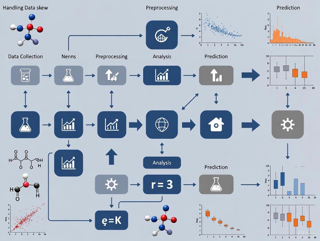
The following diagram illustrates a systematic workflow for diagnosing and treating data skew in a machine learning pipeline, integrating the concepts and protocols described above.
Diagnosis and Mitigation Workflow for Data Skew
The Scientist's Toolkit: Key Research Reagents and Solutions
This table details essential computational and methodological "reagents" for handling data skew in pharmaceutical AI research.
| Tool/Reagent | Function/Benefit | Application Context |
|---|---|---|
| Apache Spark | Distributed processing engine with built-in mechanisms (e.g., salting, adaptive query execution) to handle skewed data in large datasets [4]. | Pre-processing and model training on large-scale genomic or patient data. |
| Synthetic Data Generators (GANs) | Generates privacy-compliant, synthetic patient data to balance class distribution and mitigate bias, useful for rare disease research [6] [7]. | Augmenting training sets for rare event prediction where real data is limited. |
| Box-Cox Transform | A parameterized transformation that finds the optimal power transformation to best approximate a normal distribution [5] [8]. | Normalizing heavily right-skewed continuous features like biomarker concentrations. |
| SMOTE | An oversampling technique that creates synthetic examples for the minority class to rectify class imbalance [5] [6]. | Improving model sensitivity for detecting rare diseases or adverse drug reactions. |
| FAIR Data Principles | A framework (Findable, Accessible, Interoperable, Reusable) to ensure data quality and mitigate biases from flawed or outdated data [9]. | Foundational data governance to prevent skew issues at the source in drug discovery pipelines. |
The Critical Link Between Feature Distribution and Predictive Model Stability
Frequently Asked Questions
Q1: What is data skew and why is it a critical concern in predictive modeling for research? Data skew refers to an asymmetry in the distribution of your data where the tail of the distribution is longer on one side [10]. This is a critical concern because it can fundamentally distort analytical insights and bias machine learning models toward the majority class or dominant range of values [10] [11]. In stable predictive models, we expect features to behave consistently; skewed features violate this assumption, leading to unreliable predictions and poor generalization on new data [11] [12].
Q2: How can I quickly check if my dataset has skewed features?
You can calculate the skewness value for each feature. A value close to zero indicates a symmetrical distribution, while significant positive or negative values indicate skew [10]. The table below provides a guideline for interpretation. Python libraries like Pandas (df['column'].skew()) and visualization tools like histograms with Kernel Density Estimate (KDE) plots are essential for this initial diagnostic [13].
Table: Interpreting Skewness Values
| Skewness Value | Interpretation | Impact on Model Stability |
|---|---|---|
| Between -0.5 and 0.5 | Approximately Symmetric | Low risk; model assumptions are likely met. |
| Less than -1 or Greater than 1 | Highly Skewed | High risk; can significantly bias model outcomes and destabilize predictions. |
| Greater than 0 | Positive (Right) Skew | Most data is concentrated on the left with a long tail to the right [10]. |
| Less than 0 | Negative (Left) Skew | Most data is concentrated on the right with a long tail to the left [10]. |
Q3: My model is biased towards the majority class in a highly skewed clinical outcome variable. What can I do? This is a common issue in medical datasets, such as those with a rare disease outcome. Transforming the target variable can linearize the relationship and make it easier for models to learn effectively [14]. For a positively skewed continuous target like 'Disease Progression Score', a log transformation is often the first step. Critical Note: If you transform your target variable before training, you must apply the inverse transformation to your final predictions to get them back on the original scale for interpretation [14].
Q4: Which scaling technique should I use for my skewed features to improve model convergence? For skewed features, Robust Scaling is often the best choice because it uses the median and Interquartile Range (IQR) and is therefore resistant to outliers that are common in skewed data [15] [16]. Standardization (Z-score normalization) can also be used but is more sensitive to extreme values [15] [16]. Min-Max scaling is generally not recommended for skewed data as it is highly sensitive to outliers [15].
Table: Comparison of Feature Scaling Techniques on Skewed Data
| Technique | Formula | Best For Skewed Data? | Outlier Sensitivity |
|---|---|---|---|
| Robust Scaling | (Xᵢ - Median) / IQR | Yes | Low [15] |
| Standardization | (Xᵢ - Mean) / Std | Sometimes | Moderate [15] |
| Min-Max Scaling | (Xᵢ - Min) / (Max - Min) | No | High [15] |
Q5: How do I fix high skewness in a feature before training a model? Applying a power transformation is the most effective method. The choice depends on your data:
- For Positive Values with Positive Skew: Use the Log Transformation or Box-Cox Transformation [11] [13]. Box-Cox is more powerful as it finds the optimal parameter (λ) to maximize normality but requires strictly positive data [13].
- For Data with Zero or Negative Values: Use the Yeo-Johnson Transformation, which is flexible and handles both positive and negative values [11] [13].
- For a Guaranteed Normal Output: Use the Quantile Transformation, which maps your data to a specified distribution (e.g., normal) by force, effectively removing skewness [13].
Troubleshooting Guides
Problem: Model performance is poor, and feature importance shows bias towards high-magnitude features.
- Symptoms: Inaccurate predictions, unreliable insights, and the model fails to generalize on unseen data [11]. In distance-based algorithms like K-Nearest Neighbors (KNN) or K-Means, features with larger scales can overshadow others [16].
- Root Cause: The dataset contains features with significantly different scales and distributions. Skewed features can dominate the model's learning process, regardless of their true relevance [16].
- Solution:
- Diagnose: Calculate skewness for all numerical features and visualize their distributions.
- Transform: Apply a power transformation (e.g., Box-Cox, Yeo-Johnson) to highly skewed features to make their distributions more symmetrical [13].
- Scale: Use Robust Scaling or Standardization on all features to ensure they contribute equally to the model [15] [16].
- Re-train & Validate: Re-train the model on the transformed and scaled dataset and validate its stability on a hold-out test set.
Problem: Gradient-based models (e.g., Neural Networks, Linear Regression) are converging slowly or unstably.
- Symptoms: The training process is erratic, the loss function fluctuates widely, and the model takes a long time to converge to a minimum.
- Root Cause: Features are on vastly different scales. This causes gradients to update at different rates, making the optimization path inefficient and unstable [16].
- Solution:
- Standardize Features: Apply Standardization (Z-score normalization) to transform features to have a mean of 0 and a standard deviation of 1 [15] [16]. This is particularly crucial for algorithms like Linear Regression and Neural Networks [16].
- Monitor Training: Use learning curves to monitor the loss and validation metrics during training after standardization to confirm improved stability.
Experimental Protocol: Correcting for Data Skew
This protocol outlines a systematic approach to diagnose and correct feature skew to enhance predictive model stability.
1. Hypothesis: Correcting for skewness in feature distributions through appropriate transformations will improve model stability and predictive performance.
2. Experimental Workflow: The following diagram illustrates the key steps for diagnosing and treating data skew in a modeling pipeline.
3. Detailed Methodology:
- Step 1: Diagnose Skewness
- Procedure: For each numerical feature, calculate the skewness coefficient using a function like
pandas.DataFrame.skew(). Visually inspect distributions using histograms with KDE plots [13]. - Decision Threshold: Typically, a skewness value greater than 0.5 or less than -0.5 warrants investigation, and values beyond 1 or -1 almost certainly require correction [10].
- Procedure: For each numerical feature, calculate the skewness coefficient using a function like
Step 2: Apply Transformation
Step 3: Scale Features
- Procedure: After correcting skewness, scale the features. Use a
RobustScalerif outliers are suspected, or aStandardScalerotherwise [15]. Always fit the scaler on the training data and use it to transform both training and test sets.
- Procedure: After correcting skewness, scale the features. Use a
Step 4: Validate Stability
- Metrics: Compare the model's performance on validation/test sets before and after treatment. Look for improvements in metrics like R², Mean Absolute Error (MAE), and the stability of feature importance rankings across different data splits.
The Scientist's Toolkit
Table: Essential Research Reagents for Data Stability Experiments
| Reagent / Tool | Function / Explanation |
|---|---|
| Pandas Library | Foundational Python library for data manipulation and analysis; used to calculate descriptive statistics and handle dataframes. |
| Scikit-learn Preprocessing | Provides ready-to-use scalers (StandardScaler, RobustScaler) and transformers (PowerTransformer) for consistent data treatment [15] [13]. |
| SciPy Stats Library | Offers advanced statistical functions, including the boxcox and yeojohnson transformations for normality [13]. |
| Seaborn/Matplotlib | Visualization libraries used to plot feature distributions (histograms, KDE plots) before and after transformation to visually assess effectiveness [13]. |
| Robust Scaler | A scaling reagent that uses median and IQR, making it essential for pre-processing datasets with outliers or heavy skews [15]. |
FAQs on Batch Effects
Q1: What are batch effects and why are they a critical problem in biomedical data analysis?
Batch effects are technical variations introduced into high-throughput data due to factors unrelated to the study's biological objectives. These can arise from variations in experimental conditions over time, using different laboratories or machines, or employing different analysis pipelines [17]. They are critically important because they can introduce noise that dilutes true biological signals, reduce statistical power, and potentially lead to misleading, biased, or non-reproducible results [17]. In severe cases, batch effects have been identified as a paramount factor contributing to the reproducibility crisis in science, resulting in retracted articles, invalidated research findings, and significant economic losses [17].
Q2: At what stages of an experiment can batch effects be introduced?
Batch effects can emerge at virtually every step of a high-throughput study [17]. Common sources include:
- Study Design: Flawed or confounded design where samples are not collected randomly or are selected based on specific characteristics.
- Sample Preparation & Storage: Variations in protocols, such as different centrifugal forces during plasma separation or differences in storage temperature and duration.
- Data Generation: Using different machines, instruments, or reagent batches.
- Data Processing: Utilizing different bioinformatic pipelines for analysis.
Q3: What is the difference between a balanced and a confounded study design, and why does it matter for batch correction?
The ability to correct for batch effects depends heavily on the initial experimental design [18].
- In a balanced design, the phenotype classes of interest are equally distributed across the different batches. In this scenario, batch effects may be "averaged out" when comparing phenotypes.
- In a confounded design (or fully imbalanced design), the phenotype classes separate completely by batch. Here, the phenotype perfectly correlates with the batch, making it nearly impossible to distinguish whether observed differences are due to true biology or technical artifacts [18]. Correction in confounded designs is challenging and sometimes not possible.
Q4: How can I evaluate the performance of a Batch Effect Correction Algorithm (BECA) for my dataset?
Simply trusting visualizations like PCA plots or a single metric can be misleading [19]. A robust evaluation involves:
- Downstream Sensitivity Analysis: Compare the outcomes (e.g., lists of differentially expressed features) obtained from analyzing batches individually versus after applying a BECA. A good BECA should help recover the "union" of true biological findings from the separate batches [19].
- Multiple Metrics: Use a variety of evaluation metrics. Be cautious of methods that rank BECAs by a single aggregated score, as a poor performance in one critical metric might be masked by good performance in others [19].
- Workflow Compatibility: Ensure the BECA is compatible with your entire data processing workflow (e.g., normalization, missing value imputation), as each step influences the next [19].
Troubleshooting Guide: Batch Effects
Problem: Clustering by batch in PCA plots.
- Potential Cause: Strong technical variation between processing groups is overshadowing biological signal.
- Solution:
- Apply a batch effect correction algorithm like ComBat or limma's
removeBatchEffect()[17] [18]. - If using proteomic data with many missing values, consider tools like HarmonizR that correct without imputation [20].
- Always check the design balance. If it is confounded, correction may not be feasible, and the data should be interpreted with extreme caution.
- Apply a batch effect correction algorithm like ComBat or limma's
- Potential Cause: Batch effects are confounding the biological interpretation, or "Batch Effect Associated Missing Values (BEAMs)" are skewing the analysis [21].
- Solution:
- Detect BEAMs: Identify features that are entirely missing in one batch but present in another.
- Handle BEAMs Carefully: Standard missing value imputation (MVI) methods perform poorly on BEAMs, often introducing artifacts [21]. Avoid using KNN, SVD, or Random Forest imputation directly on such data without considering batch structure.
- Use Batch-Aware Methods: Employ a batch-sensitized MVI strategy or a unified pipeline that handles both MVI and BEC appropriately [21].
Problem: A previously identified biomarker fails to validate in a new batch.
- Potential Cause: The original "biomarker" was actually a artifact of batch effects in the discovery dataset [17] [22].
- Solution:
- Re-analyze the original data using quality-aware batch correction methods to verify the signal is truly biological [22].
- In future studies, implement a study design that balances biological groups across batches from the outset.
- Use machine learning quality scores to assess and account for batch-related quality differences during analysis [22].
FAQs on Rare Events
Q1: What defines a "rare event" in biomedical data?
Rare events are incidents that stand out due to their infrequency, and their definition can be context-dependent [23]. In machine learning for biomedical data, this often refers to a significant class imbalance where the event of interest (e.g., a circulating tumor cell) is vastly outnumbered by other events (e.g., regular blood cells) [24] [23]. The "Curse of Rarity" (CoR) describes the challenge that these events provide limited information due to their scarcity, leading to issues in decision-making, modeling, and validation [23].
Q2: What are common approaches for detecting rare events in an unsupervised manner?
Unsupervised detection does not require prior knowledge of the rare event's signature. One effective approach uses a Denoising Autoencoder (DAE) [24].
- Principle: The DAE is trained to reconstruct clean data from a noisy version. It learns the distribution of common events very well. When a rare event is input, the reconstruction error is high because the event does not fit the common pattern. This reconstruction error serves as a metric for rarity [24].
- Workflow: The data (e.g., an image) is split into tiles. Each tile is noised and fed into the DAE. The reconstruction error is calculated for each tile, and tiles are ranked by this error, with the highest errors corresponding to the most rare (and potentially most interesting) events [24].
Troubleshooting Guide: Rare Events
Problem: A model fails to learn or identify rare biological events.
- Potential Cause: Extreme class imbalance, where the rare events are outnumbered by common events by several orders of magnitude (e.g., 1 in 1 million) [24].
- Solution:
- Data-Level Approaches: Use techniques like oversampling the rare class or undersampling the common class to create a more balanced training set [23].
- Algorithm-Level Approaches: Employ cost-sensitive learning, where a higher penalty is assigned to misclassifying the rare event, or use ensemble methods designed for imbalanced data [23].
- Anomaly Detection: Frame the problem as unsupervised anomaly detection using methods like the DAE-based RED algorithm to isolate rare events without pre-labeled data [24].
FAQs on Measurement Artifacts
Q1: How do missing values act as a measurement artifact, and what is special about BEAMs?
Missing Values (MVs) are a common artifact in high-dimensional biomedical data. They can be technically driven (e.g., below detection limit) or biologically driven (e.g., the analyte is absent) [21]. Batch Effect Associated Missing Values (BEAMs) are a specific, problematic type of MV where an entire feature (e.g., a protein or gene) is missing in one batch but present in others due to differences in platform coverage or sensitivity [21]. BEAMs present a substantial challenge because they create a perfect confounding between the batch and the missingness pattern.
Q2: How should I handle missing values in a multi-batch dataset?
The standard practice of performing Missing Value Imputation (MVI) first, followed by Batch Effect Correction (BEC), is flawed and can be detrimental when BEAMs are present [21].
- Recommended Strategy: The handling of MVs and BEC must be considered together. For standard MVs, a batch-sensitized imputation (imputing within batches) is recommended [21].
- For BEAMs: Specialized tools or cautious workflows are needed. Simply imputing values for a feature that is entirely missing in a batch can introduce false signals and artificial confidence [21]. Tools like HarmonizR, which performs batch correction on sub-matrices without imputing BEAMs, can be a more reliable approach for proteomic data [20].
Experimental Protocols
Protocol 1: Quality-Aware Batch Effect Detection and Correction in RNA-seq Data
This protocol uses a machine-learning-based quality score to detect and correct for batches without prior knowledge [22].
Quality Score Calculation:
- Input: FASTQ files.
- Tool:
seqQscoreror similar. - Method: Derive quality features from the files (either full files or a subset of 1 million reads to save time). Use a pre-trained classifier to predict a probability score (
Plow) for each sample being of low quality [22].
Batch Detection:
- Statistically compare the distribution of
Plowscores across suspected or documented batches (e.g., using Kruskal-Wallis test). A significant difference indicates that batch effects are correlated with sample quality [22].
- Statistically compare the distribution of
Batch Correction:
- Use the
Plowscore as a covariate in a correction model (e.g., in thesvapackage) to remove the variation associated with quality differences [22]. - Evaluation: Compare PCA plots and clustering metrics (Gamma, Dunn1, WbRatio) before and after correction. The goal is for samples to cluster by biological group, not by batch or quality score [22].
- Use the
Protocol 2: Unsupervised Rare Event Detection in Liquid Biopsy Images
This protocol details the use of a Denoising Autoencoder (DAE) to find rare cells in immunofluorescence images without prior labeling [24].
Image Tiling:
- Divide a large immunofluorescence image (e.g., with DAPI, Cytokeratin, Vimentin, CD45/CD31 channels) into smaller tiles of 32x32 pixels. This typically generates millions of tiles from a single image [24].
DAE Training:
- Architecture: A deep learning model with an encoder (compresses the input tile) and a decoder (reconstructs the tile).
- Training: Input noisy versions of the tiles. Train the DAE to output the clean, original tile. The model learns the distribution of common events (e.g., immune cells) present in the majority of tiles [24].
Rarity Scoring and Ranking:
- Input: Pass each clean tile through the trained DAE.
- Calculation: For each tile, compute the reconstruction error (e.g., mean squared error) between the DAE's output and the original input.
- Output: Rank all tiles based on this error. The tiles with the highest error are the most "rare" as the model could not reconstruct them well. These are candidate tiles containing biologically interesting, rare cells like CTCs [24].
Key Data Summaries
Table 1: Common Batch Effect Correction Algorithms (BECAs) and Their Characteristics
| Algorithm | Main Principle | Key Application Context | Pros | Cons |
|---|---|---|---|---|
| ComBat [17] [19] | Empirical Bayes framework to standardize mean and variance across batches. | Bulk omics data (e.g., transcriptomics, proteomics) with known batch factors. | Effective for known batches; can handle parametric and non-parametric data. | Assumes batch effects fit a linear model; requires features to be present in all batches for standard use. |
| limma's removeBatchEffect() [19] [18] | Linear model to remove batch-associated variation. | Balanced designs in bulk omics data. | Simple, fast, and effective for linear, additive effects. | Less effective for complex, non-linear batch effects. |
| HarmonizR [20] | Uses ComBat/limma on sub-matrices created by matrix dissection. | Proteomic data with extensive missing values (including BEAMs). | Does not require data imputation, preventing the introduction of imputation artifacts. | More computationally complex than standard ComBat. |
| SVA/RUV [19] | Identifies and adjusts for surrogate variables or unwanted variation. | When sources of batch effects are unknown or unrecorded. | Does not require prior knowledge of batch factors. | Risk of removing biological signal if surrogate variables are correlated with biology. |
| Rarity Level | Event Frequency | Description & Challenges |
|---|---|---|
| R1: Extremely Rare | 0 - 1% | The most challenging level. Events are exceptionally scarce, leading to the "Curse of Rarity" with very limited information for modeling. |
| R2: Very Rare | 1 - 5% | Very infrequent events. Standard ML models often ignore this class without specialized techniques (e.g., oversampling, cost-sensitive learning). |
| R3: Moderately Rare | 5 - 10% | Manageable imbalance. Ensemble methods and careful sampling can be effective. |
| R4: Frequently-Rare | > 10% | The least severe level of imbalance. Standard algorithms may perform adequately but can still benefit from imbalance-aware techniques. |
Visual Workflows and Pathways
Diagram 1: Batch Effect Assumption Model
Diagram Title: Theoretical Assumptions of Batch Effects
Diagram 2: Rare Event Detection Workflow
Diagram Title: Unsupervised Rare Event Detection Pipeline
Diagram 3: Impact of Missing Value Imputation on Batch Effects
Diagram Title: BEAMs Skew Downstream Analysis
The Scientist's Toolkit: Research Reagent Solutions
Table 3: Essential Computational Tools for Managing Data Skew
| Tool / Resource | Function | Key Application Note |
|---|---|---|
| ComBat [17] [19] | Batch Effect Correction Algorithm | Best for known batches in balanced designs. Use non-parametric mode for non-Gaussian data. |
| HarmonizR [20] | Data Harmonization Tool | Essential for proteomic datasets with high rates of missing values; avoids error-prone imputation. |
| limma R Package [19] [18] | Linear Models for Microarray & RNA-seq Data | Its removeBatchEffect() function is a fast, standard choice for linear batch effect removal. |
| seqQscorer [22] | Machine Learning-Based Quality Assessment | Automatically evaluates NGS sample quality from FASTQ files; can be used to detect quality-associated batch effects. |
| Denoising Autoencoder (DAE) [24] | Unsupervised Rare Event Detection | Framework for isolating rare analytes (e.g., CTCs) in images without prior knowledge of their signature. |
| OpDEA [19] | Workflow Sensitivity Analysis | Evaluates how sensitive differential expression results are to the choice of BECA and other workflow steps. |
Stability testing is a critical component of pharmaceutical development, essential for understanding how the quality of a drug substance or product changes over time under various environmental conditions. The International Council for Harmonisation (ICH) has provided the global benchmark for these activities for decades. A significant evolution is underway with the new ICH Q1 Step 2 Draft Guideline, endorsed in April 2025, which consolidates previous guidelines (Q1A-F and Q5C) into a single, modernized framework [25] [26] [27].
This revised guideline emphasizes science- and risk-based approaches, aligning with modern Quality by Design principles and encouraging robust stability lifecycle management [26] [27]. For researchers, this shift is paramount. It moves stability testing from a box-ticking regulatory exercise to an integrated, data-driven process that requires sophisticated handling of complex data, including navigating the challenges of data skew and feature distribution stability in prediction models.
Frequently Asked Questions (FAQs)
1. What is the most significant change in the new ICH Q1 draft guideline? The most significant change is the consolidation of multiple previous guidelines into a single, unified document. This new draft is structured into 18 main sections and 3 annexes, replacing the fragmented Q1A-F and Q5C series. It introduces a more holistic framework and expands its scope to include emerging product types like Advanced Therapy Medicinal Products (ATMPs) and provides new guidance on stability modeling and risk-based approaches [25] [26] [27].
2. How can I justify a reduced stability study design, like bracketing or matrixing? The new guideline, particularly in Annex 1, provides a clearer framework for designing reduced stability studies using bracketing and matrixing. Justification must be based on prior knowledge and robust risk assessment. For instance, bracketing (testing only the extremes of certain design factors) is acceptable when supported by data from development studies that demonstrate a clear understanding of the product's stability behavior [27].
3. My stability data is highly skewed and does not follow a normal distribution. How does this impact my shelf-life calculation? Skewed data directly challenges the traditional statistical models that often assume normality. The new guideline's Annex 2 on stability modeling acknowledges this by encouraging the use of more flexible statistical approaches. In such cases, you may need to:
- Explore Alternative Distributions: Utilize statistical models based on non-normal, or skew distributions, which offer increased flexibility for modeling asymmetric data [28] [29].
- Leverage Advanced Modeling: Employ modern machine learning techniques that can better handle distributional shifts and skewed data, ensuring more accurate and reliable shelf-life predictions [30].
4. What are the new requirements for stability studies on Advanced Therapy Medicinal Products (ATMPs)? Annex 3 of the new guideline is dedicated to ATMPs, such as cell and gene therapies. It addresses their unique stability challenges, which often include very short shelf-lives and high sensitivity. The guidance requires real-time stability assessments and considers the unique quality attributes of these complex products, though some stakeholders have noted that further detailed guidance may still be needed [25] [27].
Troubleshooting Guides
Problem 1: Handling Skewed and Multi-Modal Stability Data
Challenge: The distribution of your stability data (e.g., for a degradation product) is highly skewed or shows multiple peaks (multi-modal), violating the assumptions of standard statistical models used for shelf-life estimation [28].
Solutions:
- Utilize Flexible Statistical Distributions: Move beyond normal distribution assumptions. Consider using a Modified Generalized Skew (MGS) distribution, which can model asymmetric data with multiple modes by incorporating higher-order moments like skewness and kurtosis [28]. The density function for such a family is given by
fY(y,α,λ) = 2/(1+αρ4) * (1+αy^4) * h(y) * G(λy), whereαandλcontrol the modes and skewness [28]. - Implement Skew-Probabilistic Neural Networks (SkewPNN): For a machine learning approach, use SkewPNN. It replaces the standard Gaussian kernel in a Probabilistic Neural Network with a skew-normal kernel function, providing the flexibility to model underlying class densities in imbalanced or non-symmetric data effectively [29].
- Adopt Exact Feature Distribution Matching (EFDM): If treating lighting or environmental conditions as a style factor, use EFDM as a loss objective. This aligns the feature distributions of your data with the target distribution across multiple moments—mean, variance, skewness, and kurtosis—leading to more robust predictions in complex, multi-illuminant scenarios [30].
Experimental Protocol: Fitting a Modified Generalized Skew Distribution
- Data Collection: Collect stability data for the critical quality attribute (CQA) of interest.
- Distribution Fitting: Fit the MGS distribution to your data by estimating parameters
α(mode controller) andλ(skewness controller). - Model Selection: Compare the goodness-of-fit of the MGS distribution against the normal and standard skew-normal distributions using criteria like AIC or BIC.
- Moment Calculation: Calculate the first four moments of the fitted distribution using the provided formulas [28]:
- First moment (Mean):
μ1 = [ρ1 + αρ5] / [1 + αρ4] - Second moment (Variance related):
μ2 = [ρ2 + αρ6] / [1 + αρ4] - Third moment (Skewness related):
μ3 = [ρ3 + αρ7] / [1 + αρ4] - Fourth moment (Kurtosis related):
μ4 = [ρ4 + αρ8] / [1 + αρ4]whereρris the r-th moment of a base skew distribution.
- First moment (Mean):
- Shelf-life Estimation: Use the fitted and validated MGS model to estimate the shelf-life, ensuring the confidence intervals account for the data's specific distribution shape.
Problem 2: Adjusting to the New Guideline's Emphasis on Risk and Lifecycle Management
Challenge: Your existing stability protocols and Standard Operating Procedures (SOPs) are designed for the old, fragmented guidelines and are not aligned with the new emphasis on science- and risk-based lifecycle management.
Solutions:
- Gap Analysis: Conduct a thorough review of the entire draft guideline against your current stability procedures [25].
- Update Training and SOPs: Begin developing new training modules and updating internal SOPs to reflect the consolidated structure and new concepts, such as lifecycle stability management (Section 15) [25] [27].
- Engage Early with Regulators: Monitor communications from the FDA and EMA for evolving interpretations. Participate in industry forums to anticipate inspector expectations regarding the justification for risk-based decisions [25].
Structured Data Tables
Table 1: Comparison of Key Changes in ICH Q1 Guideline
| Aspect | Previous Guidelines (Q1A-F, Q5C) | New 2025 Draft Q1 Guideline |
|---|---|---|
| Structure | Multiple fragmented documents | Single, consolidated document (18 sections, 3 annexes) [25] [26] |
| Core Approach | Largely fixed and descriptive | Science- and risk-based, aligned with QbD [27] |
| Product Scope | Primarily synthetics and some biologics | Expanded to include ATMPs, novel excipients, drug-device combinations [27] |
| Statistical Modeling | Limited and vague guidance | New, clearer guidance in Annex 2 [25] |
| Lifecycle Management | Not explicitly addressed | Dedicated section (Section 15) on stability lifecycle management [27] |
| Reduced Designs | Addressed in Q1D | Refined and incorporated into Annex 1 with emphasis on risk-justification [27] |
Table 2: Research Reagent Solutions for Stability Studies
| Item | Function in Stability Prediction |
|---|---|
| Reference Standards | Essential for ensuring the reliability and consistency of analytical methods throughout the stability study. The new guideline provides clearer instructions on their stability testing and storage [25]. |
| Novel Excipients/Adjuvants | These can significantly impact product stability. The guideline now includes specific considerations for their evaluation due to their potential effect on drug product quality [26] [27]. |
| Validated Modeling Software | Critical for implementing the statistical modeling and predictive stability approaches encouraged in Annex 2 of the new guideline. Used for shelf-life prediction and extrapolation [25]. |
| Forced Degradation Samples | Samples deliberately degraded under extreme conditions (e.g., high heat, pH, oxidation) are key reagents for validating stability-indicating analytical methods during development studies [26] [27]. |
Workflow and Relationship Diagrams
Stability Study Design Workflow
Handling Skewed Data in Stability Prediction
Technical Support & Troubleshooting Guides
Frequently Asked Questions (FAQs)
Q1: My AI model for predicting compound efficacy performs well in validation but fails in real-world testing. What could be wrong?
A: This is a classic symptom of data skew undermining model generalizability. The most likely cause is a covariate shift, where the statistical distribution of the input features (e.g., chemical structures, assay data) in your real-world data differs from the data used to train and validate the model [31]. For instance, your training data may overrepresent certain molecular scaffolds, causing the model to perform poorly on novel chemotypes encountered in production.
- Diagnosis Checklist:
- Compare the distributions of key molecular descriptors (e.g., molecular weight, logP, polar surface area) between your training set and the new, real-world data.
- Perform a Principal Component Analysis (PCA) to visualize if the new data clusters outside the domain of your training data.
- Audit your data collection process for sampling bias, where the training data was not representative of the entire chemical space of interest due to experimental priorities or technical limitations [32].
Q2: My dataset for a toxicity prediction model has very few positive (toxic) compounds. The model has high overall accuracy but misses all the toxicants. How can I fix this?
A: You are dealing with a class imbalance problem, a common form of data skew in drug discovery where inactive or safe compounds significantly outnumber active or toxic ones [32]. Models trained on such data become biased toward the majority class.
- Solution Pathway:
- Do not rely on accuracy alone. Use metrics like Precision, Recall (Sensitivity), and the F1-score, which are more informative for imbalanced datasets [33].
- Apply resampling techniques: Use Synthetic Minority Over-sampling Technique (SMOTE) to generate synthetic samples of the minority (toxic) class. This technique creates new data points by interpolating between existing minority class instances in feature space, helping to balance the dataset and refocus the model [32].
- Consider algorithmic solutions: Use models like Cost-Sensitive Classifiers that impose a higher penalty for misclassifying the minority class during training.
Q3: After deploying a model for high-throughput screening, the results are inconsistent with subsequent manual assays. The Z'-factor was acceptable. What should I investigate?
A: While a good Z'-factor indicates a robust assay window, it does not guarantee that the data distribution fed into your model is stable [34]. The issue may lie in technical bias introduced during data processing.
- Troubleshooting Steps:
- Verify data normalization: Ensure that the method used to normalize signals (e.g., using ratiometric data analysis in TR-FRET assays) is applied consistently and correctly. Small lot-to-lot variability in reagents can affect raw signals but should be corrected by proper ratiometric calculations [34].
- Check for instrumentation drift: Confirm that the instrument settings (e.g., laser power, detector gain) have not drifted over time, as this can introduce a subtle covariate shift.
- Audit the feature engineering pipeline: Ensure that the steps for calculating molecular features from raw data are identical between the development and deployment phases.
The following table summarizes quantitative findings from studies investigating data skew and model performance in biomedical contexts.
Table 1: Impact of Data Skew and Mitigation Strategies on Model Performance
| Study Context | Skew Type / Mitigation Method | Key Performance Finding | Citation |
|---|---|---|---|
| Sepsis Early Detection Model (First Affiliated Hospital of Zhengzhou University) | Integration of MLD with EHR to address data representativeness. | Model sensitivity: 87%; specificity: 89%, significantly outperforming traditional methods. [35] | |
| Ovarian Cancer Diagnostic Models | Comparative analysis of models on blood test data. | Best-performing model (Medina, Jamie E. et al.) achieved sensitivity of 0.91 and specificity of 0.96 on training set. [35] | |
| Polymer Material Property Prediction | Use of SMOTE to balance imbalanced data. | Application of SMOTE with XGBoost improved the prediction of mechanical properties in an imbalanced dataset. [32] | |
| Catalyst Design for Hydrogen Evolution | Use of SMOTE to address uneven data distribution. | SMOTE improved predictive performance of ML models for candidate screening. [32] | |
| General Model Assessment | Z'-factor for assay quality (not model quality). | Assays with Z'-factor > 0.5 are considered suitable for screening. A large assay window with high noise can have a lower Z'-factor than a small window with low noise. [34] |
Experimental Protocols
Protocol 1: Detecting Covariate Shift in a Compound Library
Objective: To determine whether new, externally sourced compounds fall outside the feature distribution of a model's training set.
Materials: Training dataset, new compound dataset, chemical descriptor calculation software (e.g., RDKit).
Methodology:
- Calculate Descriptors: For both training and new compound sets, calculate a standardized set of molecular descriptors (e.g., MW, logP, number of rotatable bonds, H-bond donors/acceptors).
- Standardize Data: Apply the same scaling (e.g., StandardScaler) fitted only on the training data to both sets.
- Dimensionality Reduction: Perform PCA on the scaled training data. Project the new data onto the same principal components.
- Visualization & Analysis: Create a scatter plot of the first two principal components (PC1 vs. PC2). Visually inspect if the new compounds cluster within the cloud of training data.
- Quantitative Measure: Calculate the Mahalanobis distance (or use a population stability index) between the training and new datasets in the principal component space. A large distance indicates a significant covariate shift. [31]
Protocol 2: Mitigating Class Imbalance with SMOTE
Objective: To balance a dataset for a toxicity prediction model where toxic compounds are the minority class.
Materials: Imbalanced dataset, programming environment (e.g., Python) with imbalanced-learn library.
Methodology:
- Data Preprocessing: Split data into features (X) and target (y). Perform train-test split before applying SMOTE to avoid data leakage.
- Apply SMOTE: Apply the SMOTE algorithm exclusively to the training data. SMOTE generates synthetic minority class samples by:
- For each sample in the minority class, finding its k-nearest neighbors (typically k=5).
- Selecting one of these neighbors at random.
- Calculating a synthetic data point at a random point on the line segment connecting the original sample and its selected neighbor. [32]
- Model Training: Train your classifier (e.g., Random Forest, XGBoost) on the resampled, balanced training set.
- Validation: Evaluate the model on the untouched, imbalanced test set using metrics like AUC-PR and F1-score.
The workflow for this protocol is outlined below.
The Scientist's Toolkit: Research Reagent Solutions
Table 2: Essential Resources for Managing Data Skew in Drug Discovery
| Item / Solution | Function / Description | Relevance to Skew & Generalizability |
|---|---|---|
| SMOTE & Variants (Borderline-SMOTE, SVM-SMOTE) | Algorithmic oversampling techniques to synthetically generate samples for the minority class. [32] | Directly addresses class imbalance, preventing model bias toward the majority class and improving prediction of rare outcomes (e.g., toxicity, high-efficacy). |
| Explainable AI (xAI) Tools (e.g., SHAP, LIME) | Provides post-hoc interpretations of model predictions, highlighting the most influential features. [36] | Uncovers hidden biases by revealing if models rely on spurious correlations. Increases trust and allows researchers to audit and refine models. |
| Federated Learning Frameworks | A distributed learning technique where models are trained across multiple decentralized data sources without sharing the raw data. [35] | Mitigates sample selection bias by leveraging more diverse datasets from different institutions, leading to more robust and generalizable models. |
| Z'-Factor Statistical Metric | A measure of the quality and robustness of an assay, incorporating both the assay dynamic range and the data variation. [34] | Ensures high-quality, reproducible input data. Poor assay quality (low Z'-factor) is a source of noise and bias that propagates through the ML pipeline. |
| Hash-Based Partitioning | A data management technique to ensure even distribution of data across computational partitions in distributed systems. [37] | Prevents technical data skew during large-scale processing, ensuring efficient model training and preventing bottlenecks that can distort analysis. |
Methodological Approaches: Data Resampling, ASAP, and ML for Stability Modeling
Frequently Asked Questions (FAQs)
Q1: Why is accuracy a misleading metric for imbalanced datasets, and what should I use instead? In imbalanced datasets, a model can achieve high accuracy by simply predicting the majority class for all instances. For example, in a dataset where 99% of transactions are non-fraudulent, a model that always predicts "non-fraudulent" will be 99% accurate but useless for identifying fraud [38] [39]. Instead, you should use metrics that provide a nuanced view of model performance, such as Precision, Recall, F1-score, and AUC-ROC [40] [39]. These metrics better capture the model's effectiveness at identifying the minority class.
Q2: When should I choose SMOTE over Random Undersampling for my experiment? The choice depends on your dataset size and the risk you want to mitigate.
- Use SMOTE when your overall dataset is not extremely large, and you want to avoid losing information. SMOTE is preferred as it generates new synthetic samples for the minority class, helping the model learn its characteristics without mere duplication [38] [41].
- Use Random Undersampling when you have a very large dataset (millions of rows) and computational efficiency is a concern. Be aware that randomly removing majority class instances can lead to a significant loss of valuable information [39].
Q3: My model is overfitting after applying SMOTE. What is the cause, and how can I resolve it? A common cause is that the standard SMOTE algorithm can generate noisy samples in the feature space or create too many synthetic instances in high-density regions of the minority class, leading the model to learn an overly specific pattern [38] [42]. Consider these solutions:
- Use Hybrid Techniques: Combine SMOTE with data cleaning methods like SMOTE + Tomek Links or SMOTE + ENN. These hybrids remove overlapping data points from both classes after oversampling, resulting in a clearer decision boundary and reduced overfitting [38].
- Try Advanced Variants: Implement improved algorithms like ISMOTE (Improved SMOTE), which expands the sample generation space to create more diverse and realistic synthetic samples, thereby better preserving the underlying data distribution [42].
Q4: How can I implement a basic SMOTE process in Python for a binary classification problem?
You can use the imblearn library to easily implement SMOTE. The following code snippet demonstrates the process [38]:
Remember, SMOTE should only be applied to your training set. Your test set should remain unchanged to properly evaluate model performance on the original data distribution [38].
Troubleshooting Guides
Problem: SMOTE Generates Noisy or Unrealistic Samples
Diagnosis: This occurs when synthetic samples are generated in regions that overlap with the majority class or do not conform to the true data manifold, confusing the classifier [42].
Solution:
- Switch to a Focused Oversampling Algorithm: Use Borderline-SMOTE, which only oversamples minority instances that are on the "borderline" (hard to classify) rather than all minority instances, reducing the generation of noise [42].
- Apply a Cleaning Hybrid Method: Use the SMOTETomek hybrid method from
imblearn, which applies SMOTE first and then removes Tomek links (pairs of close instances from opposite classes) to clean the feature space [38].
Problem: Significant Loss of Information After Random Undersampling
Diagnosis: Randomly discarding majority class samples can remove instances that carry important patterns, leading to an under-trained model [39].
Solution:
- Use Informed Undersampling: Instead of random removal, use methods that aim to preserve important majority samples. Tomek Links can be used for undersampling by removing only the majority class instance from each Tomek pair, which are borderline points [39].
- Implement a Hybrid Approach: Combine undersampling with SMOTE. This balances the dataset while mitigating the downsides of each method used alone. The
imblearnlibrary provides built-in hybrid methods [38]. - Apply Ensemble Undersampling: Use EasyEnsemble or BalancedRandomForest classifiers. These algorithms create multiple subsets of the majority class and ensemble the results, ensuring that different majority class samples are considered across models and reducing information loss [40].
Problem: The Classifier Still Favors the Majority Class After Resampling
Diagnosis: The resampling process might not have been sufficient, or the model needs a direct incentive to pay more attention to the minority class.
Solution:
- Adjust Class Weights: Many machine learning algorithms (e.g., in scikit-learn) have a
class_weightparameter. Setting this to'balanced'automatically adjusts weights inversely proportional to class frequencies. This makes the model penalize misclassifications of the minority class more heavily [40]. - Tune the Resampling Ratio: SMOTE and undersampling don't always require a perfect 1:1 balance. Experiment with different
sampling_strategyratios (e.g., 0.5, 0.75) to find the optimal class distribution for your specific problem [43]. - Re-evaluate Your Metrics: Ensure you are not using accuracy. Confirm that improvements in Recall (ability to find all positive samples) and F1-score (balance between precision and recall) are being observed, even if overall accuracy decreases slightly [38] [39].
Experimental Protocols & Data
Protocol 1: Benchmarking Resampling Techniques
This protocol outlines a standardized method for comparing the efficacy of different data-level solutions on a given imbalanced dataset [38] [42].
1. Data Preparation:
- Split the dataset into a fixed training set (e.g., 70%) and a test set (e.g., 30%). The test set must remain untouched and reflect the original, real-world class distribution.
- Preprocessing: Apply feature scaling and encoding based on the dataset's requirements.
2. Resampling Application (on Training Set Only):
- Apply the following techniques to the training data only:
- Baseline: No resampling.
- Random Undersampling: Reduce the majority class randomly.
- SMOTE: Generate synthetic minority class samples.
- ADASYN: A SMOTE variant that generates more samples for "hard-to-learn" minority instances [38].
- Hybrid Method (e.g., SMOTE + Tomek Links).
3. Model Training & Evaluation:
- Train the same classifier (e.g., Logistic Regression, Random Forest) on each resampled training set.
- Evaluate all models on the same, original test set.
- Record key performance metrics: Precision, Recall, F1-Score, and AUC-ROC.
4. Workflow Diagram: The following diagram visualizes the experimental workflow.
Protocol 2: Evaluating Feature Distribution Stability Post-Resampling
This protocol is crucial for thesis research focused on whether resampling distorts the original feature space and how that impacts model robustness [42] [44].
1. Dimensionality Reduction:
- Apply a technique like PCA (Principal Component Analysis) or t-SNE to the original training data (before resampling) to project it into 2 or 3 dimensions for visualization.
2. Comparative Visualization:
- Apply the same PCA/t-SNE transformation (fitted on the original data) to the resampled datasets (e.g., after SMOTE, after undersampling).
- Create 2D/3D scatter plots for the original and each resampled dataset. Visually inspect if the synthetic samples (from SMOTE) follow the natural cluster of the original minority class or if they create artificial, distorted patterns [42].
3. Quantitative Stability Metrics:
- Intra-class Distance: Calculate the average distance between minority class samples before and after resampling. A significant increase might indicate generation of noisy, spread-out samples.
- Inter-class Overlap: Measure the separation between majority and minority class distributions post-resampling. Increased overlap can signal a noisier dataset.
Performance Comparison of Resampling Techniques
The table below summarizes quantitative findings from a study comparing various oversampling algorithms across multiple public datasets, using metrics critical for imbalanced data [42].
Table 1: Classifier Performance Improvement with Different Oversampling Techniques (Average Relative % Increase)
| Oversampling Technique | F1-Score | G-Mean | AUC-ROC |
|---|---|---|---|
| ISMOTE (Improved SMOTE) | +13.07% | +16.55% | +7.94% |
| Standard SMOTE | Base | Base | Base |
| ADASYN | Lower | Lower | Lower |
| Borderline-SMOTE | Lower | Lower | Lower |
Resampling Technique Selection Guide
The table below provides a strategic overview of when to use each technique based on dataset characteristics and research goals.
Table 2: Strategic Guide to Data-Level Solutions
| Technique | Ideal Use Case | Advantages | Disadvantages & Risks |
|---|---|---|---|
| Random Undersampling | Very large datasets; computational cost is a primary concern [39]. | Simple, fast; reduces computational load. | High risk of losing valuable data from the majority class [39]. |
| SMOTE | Small to medium-sized datasets; the goal is to avoid information loss [38] [42]. | Generates diverse synthetic data; avoids mere duplication. | Can generate noisy samples and cause overfitting in high-density regions [38] [42]. |
| Hybrid (SMOTE+ENN) | Datasets with significant class overlap; stability of the feature distribution is critical [38]. | Cleans data space; leads to well-defined class clusters. | Can be too aggressive, removing too many samples. |
| Algorithm-Level (Class Weights) | A quick first solution; when using algorithms that support it (e.g., SVM, Random Forest) [40]. | No change to the dataset; easy to implement. | May be less effective than data-level methods when complex, new data patterns are needed [43]. |
Table 3: Key Software Tools and Libraries for Imbalanced Data Research
| Tool / Library | Function | Application in Research |
|---|---|---|
| Imbalanced-Learn (imblearn) | A Python library providing a wide array of resampling techniques. | The primary tool for implementing SMOTE, its variants (ADASYN, Borderline-SMOTE), undersampling, and hybrid methods in a scikit-learn compatible framework [38] [39]. |
| Scikit-learn | A core library for machine learning in Python. | Used for data preprocessing, training baseline and comparative models, and calculating all essential evaluation metrics (F1, Precision, Recall, AUC-ROC) [39]. |
| SMOTE Variants (ISMOTE, G-SMOTE) | Advanced algorithms that improve upon the standard SMOTE data generation mechanism. | Critical for research aiming to enhance the quality and realism of synthetic samples, thereby improving feature distribution stability and model generalization [42]. |
| SHAP (SHapley Additive exPlanations) | A unified framework for interpreting model predictions. | Used post-training to explain which features drive predictions for minority class instances, adding a layer of interpretability to models trained on resampled data [45]. |
Troubleshooting Guides
G1: Poor Performance on Minority Class
Problem: Your model achieves high overall accuracy but fails to identify sick patients or rare events (the minority class). Diagnosis: This is a classic symptom of class imbalance. The classifier is biased towards the majority class because it is penalized equally for all types of errors, making it easier to "ignore" the minority class. Solution: Implement a cost-sensitive learning approach. Modify the algorithm's objective function to assign a higher misclassification cost for errors on the minority class. This forces the model to pay more attention to learning the characteristics of the minority class. Unlike resampling techniques, this method does not alter the original data distribution, preserving its integrity [46].
G2: Inconsistent Results Across Different Datasets
Problem: A model that performs well on one imbalanced medical dataset (e.g., Pima Indians Diabetes) shows degraded performance on another (e.g., Cervical Cancer Risk Factors). Diagnosis: The optimal algorithm and its parameters are often dataset-dependent. According to the "no-free-lunch" theorem, no single algorithm is superior for all problems [45]. Solution: Utilize Automated Machine Learning (AutoML) frameworks, such as H2O AutoML or Lazy Predict, for model selection. These tools automatically train and evaluate a wide range of models (e.g., Gradient Boosting, Extreme Gradient Boosting, Random Forest) and their ensembles, identifying the best-performing one for your specific dataset [45].
G3: Model is Difficult to Interpret
Problem: Your cost-sensitive model makes predictions, but you cannot understand which features it relies on, which is critical for medical diagnosis. Diagnosis: Complex ensemble or neural network models can act as "black boxes." Solution: Integrate model interpretation tools into your workflow. Use methods like SHapley Additive exPlanations (SHAP) to determine the importance and contribution of each input feature to the final prediction, providing crucial insight for researchers [45].
Frequently Asked Questions (FAQs)
Q1: What is the fundamental difference between cost-sensitive learning and data resampling? Cost-sensitive learning addresses imbalance by making the algorithm itself skew-insensitive, typically by imposing a higher penalty for misclassifying minority class examples within its loss function. In contrast, resampling (like SMOTE) alters the original training data distribution by adding synthetic minority samples or removing majority samples. A key advantage of cost-sensitive learning is that it avoids potential overfitting or loss of information that can occur from manipulating the dataset [46].
Q2: For which types of algorithms can cost-sensitive learning be applied? The cost-sensitive principle can be applied to a wide range of core machine learning algorithms. Research has demonstrated successful implementations by modifying the objective functions of Logistic Regression, Decision Trees, Extreme Gradient Boosting (XGBoost), and Random Forest models [46].
Q3: How do I know what cost weights to assign to each class? There is no universal set of weights. The optimal cost ratio is typically determined through empirical experimentation, often using cross-validation on the training data. A common starting point is to set the cost for each class inversely proportional to its frequency in the training data, but these weights should be treated as hyperparameters to be tuned for optimal performance [46].
Q4: My dataset is not only imbalanced but also small. What should I do? For small, imbalanced datasets, rigorous validation is crucial. Use stratified k-fold cross-validation to ensure that each fold preserves the class distribution of the overall dataset. This provides a more reliable estimate of model performance than a simple train-test split. Furthermore, consider leveraging ensemble methods or AutoML techniques that are effective even with limited data [45].
Q5: How can I ensure my model's predictions are stable and reliable for clinical use? Stability and reliability are achieved through a robust validation framework. This includes:
- Using multiple, independent medical datasets for validation [46].
- Reporting performance metrics specifically for the minority class (e.g., sensitivity, F1-score) in addition to overall accuracy.
- Performing statistical significance tests to compare different algorithmic approaches [46] [45].
- Interpreting model decisions with tools like SHAP to ensure they align with clinical knowledge [45].
Experimental Protocols & Data
Protocol: Validating a Cost-Sensitive Classifier on Medical Data
Objective: To compare the performance of a standard classifier against its cost-sensitive version on an imbalanced medical dataset.
Materials:
- Dataset: One of the benchmark medical datasets (e.g., Pima Indians Diabetes, Haberman Breast Cancer) [46].
- Algorithms: Standard and cost-sensitive versions of Logistic Regression, Decision Tree, and XGBoost.
- Evaluation Metrics: Accuracy, Sensitivity (Recall), Specificity, F1-Score.
Methodology:
- Data Preparation: Split the data into 70% training and 30% test sets, using stratification to maintain the imbalance ratio.
- Baseline Training: Train the standard (cost-insensitive) versions of the algorithms on the training set.
- Cost-Sensitive Training: Train the cost-sensitive versions. For example, set the
class_weightparameter in Scikit-learn to 'balanced' or manually tune the cost matrix. - Evaluation: Predict on the test set and calculate the evaluation metrics for both the overall model and the minority class.
- Comparison: Statistically compare the results to determine if the cost-sensitive approach yields a significant improvement in sensitivity without unduly compromising specificity.
Table 1: Example Performance Comparison on Chronic Kidney Disease Dataset (Illustrative Values)
| Algorithm | Overall Accuracy | Sensitivity (Sick Patients) | Specificity (Healthy Patients) | F1-Score (Minority Class) |
|---|---|---|---|---|
| Standard Logistic Regression | 92% | 65% | 97% | 0.70 |
| Cost-Sensitive Logistic Regression | 90% | 85% | 91% | 0.82 |
| Standard Decision Tree | 89% | 60% | 95% | 0.65 |
| Cost-Sensitive Decision Tree | 88% | 82% | 89% | 0.80 |
| Standard XGBoost | 94% | 75% | 98% | 0.78 |
| Cost-Sensitive XGBoost | 93% | 89% | 94% | 0.87 |
Note: Based on experimental results from [46].
Table 2: Characteristics of Medical Datasets Used in Imbalanced Learning Research
| Dataset | Majority Class | Minority Class | Approximate Imbalance Ratio | Key Predictors |
|---|---|---|---|---|
| Pima Indians Diabetes | Healthy | Diabetic | 1.6:1 | Glucose, BMI, Age |
| Haberman Breast Cancer | Survived ≥5 years | Died <5 years | 2.7:1 | Age, Year of Operation, Nodes |
| Cervical Cancer Risk Factors | Low Risk | High Risk | 7.7:1 | Number of Pregnancies, STDs, Hormonal Contraceptives |
| Chronic Kidney Disease | Not Chronic Kidney Disease | Chronic Kidney Disease | 3.6:1 | Blood Pressure, Albumin, Blood Glucose |
Note: Compiled from information in [46].
Model Workflow and Interpretation
Workflow: Skew-Insensitive Modeling Pipeline
The following diagram illustrates a robust workflow for developing a predictive model on imbalanced data, integrating both cost-sensitive learning and model interpretation.
Interpretation: Feature Importance in Stability Prediction
After model training, tools like SHAP can be used to interpret which input parameters were most critical for the model's predictions, a technique also used in geotechnical stability prediction [45]. The diagram below visualizes this interpretation logic.
The Scientist's Toolkit
Table 3: Essential Research Reagents & Computational Tools
| Item | Function/Brief Explanation | Example Use Case |
|---|---|---|
| Benchmark Medical Datasets | Publicly available datasets with inherent class imbalance, used for model validation and benchmarking. | Pima Indians Diabetes, Haberman Breast Cancer [46]. |
| Cost-Sensitive Algorithm Variants | Modified versions of standard ML algorithms (e.g., Logistic Regression, XGBoost) whose internal objective function penalizes minority class errors more heavily. | Directly addressing class imbalance without resampling [46]. |
| AutoML Frameworks | Tools that automate the process of model selection, training, and hyperparameter tuning, saving researcher time and identifying high-performing models. | H2O AutoML, Lazy Predict [45]. |
| Model Interpretation Libraries | Software libraries that provide post-hoc explanations for model predictions, ensuring transparency and building trust. | SHAP (SHapley Additive exPlanations) [45]. |
| Stratified Cross-Validation | A resampling technique that preserves the percentage of samples for each class in every training/validation fold, crucial for reliable performance estimation on imbalanced data. | Tuning hyperparameters on the Pima Indians Diabetes dataset. |
| Performance Metrics | Evaluation metrics that are robust to class imbalance, focusing on the minority class's prediction quality. | Sensitivity, F1-Score, Precision-Recall Curves [46]. |
Implementing Accelerated Stability Assessment Program (ASAP) for Predictive Shelf-Life
Core Concepts of ASAP
What is the fundamental principle behind ASAP, and how does it differ from traditional stability testing?
The Accelerated Stability Assessment Program (ASAP) is a science-based approach designed to predict the shelf-life of drug products accurately and rapidly. Its fundamental principle relies on the isoconversion paradigm and a humidity-corrected Arrhenius equation [47] [48].
Unlike traditional stability testing, where samples are stored at fixed conditions and time points to measure the amount of degradation, ASAP fixes the level of degradation (at the specification limit) and measures the time required to reach that level under various stressed conditions. This "time to fail" or isoconversion time is the key metric used for modeling [47] [49] [50]. This approach compensates for the complex, often non-linear kinetics commonly found in solid-state drug products [48].
How does the ASAP model account for humidity, and what is the 'B' factor?
For solid dosage forms, relative humidity (RH) is a critical factor affecting stability. ASAP uses a moisture-corrected Arrhenius equation to quantitatively account for this [47] [48]:
The equation is expressed as: ln k = ln A - (Ea/RT) + B(RH) [47] [48]
Where:
- k is the degradation rate.
- A is the Arrhenius collision frequency.
- Ea is the activation energy.
- R is the gas constant.
- T is the temperature in Kelvin.
- B is the humidity sensitivity factor.
- RH is the equilibrium relative humidity.
The B-value indicates the product's sensitivity to moisture. It typically ranges from 0 (low moisture sensitivity) to 0.10 (high moisture sensitivity). A high B-value means that a small increase in relative humidity will lead to a significant decrease in shelf-life [47] [48].
Experimental Protocols & Design
What is a typical ASAP protocol for a solid oral dosage form?
A typical ASAP study involves exposing the product, without primary packaging, to a range of controlled temperature and humidity conditions. The goal is to find the time it takes to reach the specification limit (isoconversion) at each condition [47] [50]. A standard screening protocol might look like this [48]:
Table 1: Example ASAP Screening Protocol for Solid Dosage Forms [48]
| Temperature (°C) | Relative Humidity (% RH) | Typical Time (Days) |
|---|---|---|
| 50 | 75 | 14 |
| 60 | 40 | 14 |
| 70 | 5 | 14 |
| 70 | 75 | 1 |
| 80 | 40 | 2 |
It is recommended that all analyses are executed simultaneously to minimize analytical variation [47].
How do I design an ASAP study for a liquid formulation?
For solutions or parenteral medications, relative humidity is often not a relevant stress factor. The core Arrhenius equation (without the humidity term) is typically used, and the stress factor might be replaced by others, such as oxygen levels, depending on the degradation pathway [47] [51]. A study on a parenteral medication (carfilzomib) used conditions including 40°C, 50°C, and 60°C (all at 75% RH) with testing time points ranging from 1 to 21 days [51].
The workflow for designing and executing an ASAP study, from planning to shelf-life prediction, follows a systematic process as shown in the diagram below.
Data Analysis & Modeling
What are the key parameters obtained from ASAP data modeling, and how are they used?
Fitting the isoconversion time data to the humidity-corrected Arrhenius equation allows for the determination of three key parameters [47] [48] [52]:
- Activation Energy (Ea): Represents the sensitivity of the degradation reaction to temperature. Typical values for pharmaceuticals are between 10 and 45 kcal/mol [47].
- Humidity Sensitivity Factor (B): Represents the sensitivity of the degradation reaction to moisture, as described earlier.
- Collision Frequency (A): The pre-exponential factor from the Arrhenius equation.
Once these parameters are known, the model can extrapolate the degradation rate (k) at any desired storage condition (temperature and RH). The shelf-life is then calculated as the time for the critical quality attribute to reach its specification limit at that specific rate [48].
How is the goodness-of-fit of an ASAP model validated?
The quality and predictive accuracy of the ASAP model should be checked. Common approaches include [47] [51] [52]:
- Statistical Metrics: Software like ASAPprime or Luminata often provides quantitative metrics like the coefficient of determination (R²) and predictive relevance (Q²) to assess how well the experimental data fits the model [51] [52].
- Internal Validation: Using four different ASAP conditions to predict the outcome of a fifth condition. This is suitable during product development [47].
- Comparison with Long-Term Data: Comparing the ASAP prediction against actual real-time stability data. This is a powerful method for validating the model, often used for post-approval changes [47].
Troubleshooting Common Issues
What should I do if my product does not show Arrhenius behavior?
Non-Arrhenius behavior can occur and makes ASAP predictions inaccurate. This is often due to [47]:
- Physical Changes: If the product undergoes a physical change during the stressed study (e.g., melting, change from hydrate to anhydrate form), the degradation pathway at high temperatures may not be representative of the pathway at long-term conditions.
- Microenvironment Changes: Complex kinetics can arise if the API exists in multiple physical states (crystalline, amorphous, etc.) that react with different kinetics, and the proportion of these states changes with temperature.
Solution: Investigate whether a physical change is occurring. ASAP is primarily designed for chemical degradation. If a physical change is the shelf-life limiting factor, alternative predictive methods may be needed [47].
Why are my predictions inaccurate, even with a seemingly good model fit?
Inaccurate predictions can stem from several sources:
- Extrapolation of Isoconversion Point: The model is most accurate when the isoconversion point (the specification limit) is found via interpolation between data points. Predictions become less accurate if the isoconversion point is extrapolated far beyond the measured data [47].
- Insufficiently Controlled RH: For solid dosage forms, it is critical that the RH the sample is exposed to is known and controlled. If packaged product is used in the study, the internal RH must be calculated based on the moisture transfer rate of the packaging and the moisture sorption of the product [48].
- Poor Model Fit: Check the R² and Q² values. A low value may indicate errors in data input, experimental execution, or that the model is not suitable for the product [52].
Can ASAP be applied to large molecules like proteins or peptides?
No. ASAP, in its current form, is generally not applicable to large molecules such as proteins [47]. This is because not all changes in the molecular structure of a protein are irreversible, and not all structural changes affect its biological activity. The fundamental assumptions of the Arrhenius equation and the isoconversion concept may not hold for these complex molecules [47].
Essential Tools & Materials
Successful implementation of ASAP requires specific reagents, software, and laboratory equipment. The following table details key solutions for setting up an ASAP study.
Table 2: Research Reagent Solutions for ASAP Experiments
| Item / Solution | Function / Explanation | Reference |
|---|---|---|
| Saturated Salt Slurries | Used to create mini-chambers (e.g., in sealed jars) for precise control of relative humidity around samples. Different salts provide a range of specific %RH levels. | [49] [50] |
| ASAPprime GO! Kit | A study starter kit for performance qualification. Includes active tablets for stressing, pre-prepared saturated salts, and standards to verify proper laboratory and software operations. | [49] |
| ASAPprime Software | Industry-standard software for designing studies (ASAPdesign), analyzing data, determining isoconversion times, and projecting shelf-life using Monte Carlo simulations. | [47] [49] [50] |
| Luminata Software | Integrates analytical data processing (e.g., from chromatograms) with stability calculations and visualization, streamlining the entire workflow. | [52] |
| Open-Dish Samples | For solid drug products, samples are often placed openly in stability chambers to ensure direct and known exposure to the controlled relative humidity. | [47] [48] |
Regulatory Acceptance & Applications
Is ASAP accepted by regulatory authorities for market applications?
Yes, but with specific contexts. As of the latest information, ASAP has been successfully used in over 100 regulatory filings globally [49]. Its acceptance is context-dependent [47]:
- Clinical Trials & Post-Approval Changes: ASAP data has been successfully accepted by agencies like the FDA, Health Canada, and EU authorities as bridging studies or for assessing post-approval changes (e.g., process, packaging, or formulation changes) [47] [49].
- Registration (NDA): For market approval of a new drug, ASAP is currently used as supportive data rather than the sole source for determining shelf-life. It can help to reduce stability commitments but does not fully replace traditional ICH stability studies for the primary registration dossier [47].
In which stages of the drug lifecycle can ASAP be most beneficial?
ASAP can be applied throughout the drug product lifecycle to save time and resources [47] [53]:
- Development: To select the best formulation, optimize processes, understand API-excipient compatibility, and choose appropriate packaging [47].
- Clinical Supply: To set a preliminary shelf-life for clinical trial materials, often with concurrent real-time studies [47].
- Post-Approval: To manage changes (e.g., in manufacturing site, process, or formulation) by demonstrating that the stability profile remains equivalent to the original product [47] [49].
The Accelerated Stability Assessment Program (ASAP) is a scientifically rigorous approach that uses stability modeling to accurately determine the shelf-life of pharmaceutical products in significantly shorter timeframes compared to traditional methods [50]. The methodology is supported by commercially available software, ASAPprime, which has become an industry standard for these predictions [50] [54].
This case study explores the application of ASAPprime specifically for a parenteral medication, detailing the experimental protocols, data analysis techniques, and troubleshooting strategies, with particular attention to handling skewed feature distributions in stability data. This approach is vital for accelerating drug development and supporting regulatory submissions [51].
Core Concepts and Terminology
Fundamental Principles
ASAP is based on two fundamental concepts [47]:
- Isoconversion Principle: This measures the "time to failure" – the time required for a key stability parameter (e.g., a degradant) to reach its specification limit under various stress conditions. The outcome is the time to reach this limit, rather than the degradation level at a fixed time [47].
- Humidity-Corrected Arrhenius Equation: The standard Arrhenius equation is extended to include the effect of relative humidity (%RH), a critical factor for many drug products. The equation is expressed as: ln k = ln A - (Ea/RT) + B(RH) [47] Where:
ASAPprime Software Components
- ASAPdesign: A subroutine that designs an optimal experimental plan based on product knowledge, design space limitations, required data precision, and available time and samples [50].
- Main User Interface: This component is used to input experimental results and build a mathematical model of the product's behavior, providing a probability that the product will remain within specification limits under designated storage conditions [50].
Experimental Protocol: A Carfilzomib Case Study
The following protocol is adapted from a published study on a carfilzomib parenteral drug product (10 mg/mL, filled in 6 mL vials) [51].
Materials and Equipment
Table 1: Key Research Reagent Solutions and Essential Materials
| Item | Function / Description |
|---|---|
| Parenteral Drug Product | The formulation under investigation (e.g., Carfilzomib 10 mg/mL) [51]. |
| High-Purity Water | Used in the formulation and any analytical preparations; must be sterile and pyrogen-free [55]. |
| Buffering Agents | To adjust and maintain the pH of the parenteral formulation to match physiological conditions [55]. |
| Tonicity Agents | e.g., Sodium Chloride or Dextrose, to ensure the formulation is isotonic with body fluids [55]. |
| Stability Chambers | Precision chambers capable of maintaining specific temperature and humidity conditions [51]. |
| Saturated Salt Slurries | For controlling relative humidity in "mini-chambers" or jars as per the experimental design [50]. |
| Validated UHPLC Method | For quantifying the active ingredient and specific degradation products (e.g., diol impurity, ethyl ether impurity) [51]. |
Step-by-Step Methodology
Step 1: Define Stability-Indicating Parameters Identify the shelf-life determining parameters that will be monitored. In the carfilzomib study, these were the formation of diol impurity, ethyl ether impurity, and total impurities [51].
Step 2: Design the Experiment using ASAPdesign Input the product's characteristics and constraints into ASAPdesign. The software will generate an optimized experimental plan specifying the number of conditions, temperature/RH setpoints, and time points. A typical ASAP study uses 5-8 different storage conditions with temperatures ranging from 50-80°C and relative humidity from 10-75%RH [47]. For the carfilzomib study, conditions included 30°C/65% RH, 40°C/75% RH, 50°C/75% RH, and 60°C/75% RH, among others [51].
Step 3: Execute the Stability Study
- Place unpackaged product samples (to ensure known and fixed T/RH exposure) into the designated stability chambers [56].
- Remove samples at the pre-defined time points and analyze them using the validated UHPLC method [51].
- It is recommended to analyze all samples at the same time to minimize analytical variation [47].
Step 4: Determine Isoconversion Times For each stress condition, determine the time taken for the key degradant to reach its specification limit. Use interpolation rather than extrapolation for greater accuracy [47].
Step 5: Input Data into ASAPprime Enter the isoconversion times and their corresponding temperature and humidity conditions into the main ASAPprime software to build the stability model [50].
Workflow and Data Analysis
The following diagram illustrates the end-to-end process of conducting an ASAP study for a parenteral medication.
Model Validation and Assessing Data Quality
The predictive accuracy of the model is assessed using statistical parameters. The carfilzomib study used the coefficient of determination (R²) and predictive relevance (Q²), with high values indicating robust model performance [51]. The model's predictions were further validated by comparing them with actual long-term stability results using relative difference parameters [51].
Table 2: Statistical Validation of ASAP Models in a Parenteral Medication Study
| Model Type | Number of Models Suitable (out of 13) | Key Statistical Parameters | Validation Outcome |
|---|---|---|---|
| Full ASAP Model | 1 | High R² and Q² values | Reliable prediction of degradation products [51] |
| Reduced Models | 11 | High R² and Q² values | Reliable prediction of degradation products [51] |
| Two-Temperature Model | 0 (Not suitable) | Not specified | Demonstrated ineffectiveness for this product [51] |
| Three-Temperature Model | 1 (Identified as optimal) | High R² and Q² values | Most appropriate model for the parenteral medication [51] |
Troubleshooting and FAQ: Addressing Skewed Data and Other Challenges
This section addresses specific issues researchers might encounter, with a focus on challenges related to data distribution and model reliability.
Q1: Our ASAP data for a key degradant shows a highly skewed distribution, not a normal distribution. Does this invalidate our model?
A: Not necessarily. Skewed data, where one tail of the distribution is longer or fatter than the other, can distort a model's assumptions and bias predictions [57]. ASAPprime uses robust statistical modeling and Monte Carlo simulations to estimate confidence intervals, which can account for some non-ideal data distributions [47]. Furthermore, the concept of "robust averaging," where the visual system (or a model) gives more weight to items close to the mean and less weight to outliers, is a known mechanism for handling skewed feature distributions in perceptual tasks and can inspire similar approaches in data analysis [58]. If the skew is severe, investigate the cause, such as an unrepresentative degradation pathway at high stress conditions.
Q2: Under what conditions is ASAP NOT applicable for parenteral medications?
A: ASAP has specific limitations. It is primarily designed for chemical degradation and is generally not applicable for predicting physical changes (e.g., hardness, dissolution) that do not follow Arrhenius behavior [47]. It also may not be accurate for:
- Large molecule biologics (e.g., proteins, antibodies) where molecular changes may not be irreversible or may not affect activity [47].
- Formulations that undergo a physical state change (e.g., melting, hydrate formation) under the stress conditions used in the study [47].
- Degradation pathways that are pH-sensitive if the pH of the solution changes with temperature, leading to non-representative kinetics [47].
Q3: Our model's prediction does not align with our real-time stability data. What are the potential causes?
A: Misalignment can occur due to several factors:
- Non-Representative Degradation: The degradation pathways at high-stress conditions are different from those at long-term storage conditions [47]. This is a critical failure mode.
- Incorrect Isoconversion: The isoconversion point (time to spec) was extrapolated rather than interpolated, reducing accuracy [47]. The experimental design should aim to hit, but not greatly exceed, the specification limit.
- Insufficient Data Points: The study used too few temperature/humidity conditions, resulting in an underdetermined model. A minimum of 6-8 conditions is often recommended for a reliable model [56].
- Package Modeling Errors: For packaged products, the internal humidity was incorrectly calculated. ASAP studies are best performed on unpackaged product, and the packaging's protective effect is modeled separately [47].
Q4: How is regulatory acceptance for using ASAP data in submissions?
A: Regulatory acceptance is evolving. Currently:
- Early Clinical Trials: ASAP data has been accepted by the FDA, Health Canada, and EU authorities like BfArM as bridging stability data or the primary stability data for clinical trial supply, though some countries still require long-term data [47].
- Registration (Market Approval): ASAP is typically used as supportive data and is not yet a standalone replacement for traditional stability studies for setting the final shelf-life. It can help reduce post-approval stability commitments [47].
- Post-Approval Changes: This is an area of strong acceptance. ASAP has been successfully used and accepted by numerous authorities (including the USA, UK, and several EU and Middle Eastern countries) for assessing process, packaging, or formulation changes [47].
Frequently Asked Questions (FAQs)
Q1: What is data skew and why is it a critical problem in distributed computing for life sciences research?
Data skew occurs when data in a distributed computing environment is not evenly divided across partitions, causing some processing nodes to handle disproportionately large amounts of data while others remain underutilized [59]. In life sciences research, this creates severe bottlenecks during analysis of genomic sequences, clinical trial data, or molecular modeling datasets, leading to inefficient resource utilization, longer processing times, and potential system failures during critical computational experiments [10] [59].
Q2: How does the salting technique resolve data skew in distributed join operations?
Salting mitigates data skew by adding a random component (a "salt") to keys in skewed datasets before partitioning [60]. This transforms heavily skewed keys into multiple distinct keys, distributing what would be single large partitions across multiple nodes. For example, a dominant key representing a frequently occurring gene variant can be split into "variantsalt1," "variantsalt2," etc., enabling parallel processing and eliminating computational bottlenecks [60] [59]. The process involves identifying skewed keys, appending random salts, repartitioning based on salted keys, and performing joins on the transformed dataset.
Q3: When should researchers consider multimodal distribution modeling for their pharmacological data analysis?
Multimodal distributions appear in pharmacological research when data clusters around multiple distinct values, creating several peaks in the distribution curve [61] [62]. Researchers should employ multimodal modeling when analyzing: drug response patterns across different patient subpopulations, pharmacokinetic parameters with distinct metabolic profiles, biomarker measurements indicating multiple physiological states, or dose-response relationships with varying efficacy peaks. These patterns often indicate underlying subgroups requiring separate analytical consideration [62].
Q4: What are the key indicators that my distributed computing job is suffering from data skew issues?
Common indicators include: significant variance in task execution times (some tasks take much longer than others), uneven resource utilization (some nodes have high CPU/memory usage while others are idle), slow progress in specific stages of join operations, and frequent executor failures or garbage collection issues in specific partitions [60] [59]. Monitoring partition sizes and task duration metrics provides quantitative evidence of skew.
Q5: How can I determine whether my dataset follows a multimodal distribution before selecting analytical approaches?
Visualization techniques provide the most straightforward identification method. Histograms and density plots will show distinct peaks representing different modes [62]. Statistical tests for unimodality (such as Hartigan's dip test) can provide quantitative assessment. For pharmacological data, examining cluster patterns in principal component analysis (PCA) plots and identifying multiple peaks in kernel density estimation curves are effective approaches. Additionally, mixture modeling techniques can help decompose complex distributions into their component distributions [61] [62].
Troubleshooting Guides
Problem 1: Severe Performance Degradation in Genomic Data Joins
Symptoms: Join operations between genomic annotation datasets experience extreme slowdowns; some tasks run 10-100x longer than others; cluster monitoring shows uneven CPU utilization across nodes.
Root Cause: A small subset of highly common genomic regions (e.g., frequently studied genes like TP53, BRCA1) create skewed partitions in distributed datasets [59].
Resolution Protocol:
- Skew Detection: Identify skewed keys using frequency analysis (
df.groupBy("gene_id").count().orderBy('count', ascending=False)). - Salting Implementation: Apply salting to the larger dataset using explode/array method for extreme skew cases [60]:
- Broadcast Join for Smaller Dataset: If one dataset is significantly smaller, use broadcast join for the unsalted dataset.
- Validation: Verify even partition distribution (
df.rdd.getNumPartitions()anddf.rdd.glom().map(len).collect()).
Problem 2: Inaccurate Predictive Models from Skewed Pharmacological Data
Symptoms: Machine learning models for drug response prediction show biased performance; poor generalization to minority subpopulations; validation metrics differ significantly across data segments.
Root Cause: Underlying multimodal distribution in biomarker data or response variables causes standard models to favor dominant modes while poorly representing minority subgroups [62].
Resolution Protocol:
- Distribution Analysis: Create histogram and density plots of all input features and target variables.
- Multimodal Identification: Apply statistical tests for multimodality (Hartigan's dip test, Silverman's test).
- Stratified Sampling: Implement sampling strategies that maintain representation across all modes.
- Mixture Modeling: Employ Gaussian Mixture Models or other finite mixture models to capture subpopulations.
- Ensemble Methods: Develop separate models for different modes with ensemble integration.
Problem 3: Resource Exhaustion During Large-Scale Molecular Dynamics Analysis
Symptoms: Executor memory errors during molecular trajectory analysis; frequent garbage collection pauses; failed tasks in specific stages of processing.
Root Cause: Uneven distribution of molecular interaction calculations, with certain high-interaction regions creating memory pressure on specific nodes.
Resolution Protocol:
- Memory Monitoring: Implement partition-level memory tracking.
- Dynamic Salting: Apply salting with appropriate salt count based on skew ratio:
- Data Repartitioning: Use
repartition()orcoalesce()with salted keys to balance load. - Executor Configuration: Increase executor memory or reduce cores per executor for stability.
Table 1: Data Skew Impact on Distributed Processing Performance
| Skew Ratio | Task Time Variance | Cluster Utilization | Recommended Salt Count |
|---|---|---|---|
| < 2:1 | Low (< 20%) | Balanced (> 85%) | 0 (No salting needed) |
| 2:1 - 5:1 | Moderate (20-50%) | Slight imbalance (70-85%) | 2-5 |
| 5:1 - 10:1 | High (50-100%) | Significant imbalance (50-70%) | 5-10 |
| > 10:1 | Severe (> 100%) | Highly inefficient (< 50%) | 10-20 |
Table 2: Multimodal Distribution Characteristics in Pharmacological Research
| Distribution Type | Common Occurrences | Recommended Analytical Approach | Statistical Considerations |
|---|---|---|---|
| Bimodal | Drug responder vs. non-responder populations; Fast vs. slow metabolizers | Finite mixture models, Stratified analysis | Mean misleading; report modes separately; Consider skewness within modes [62] |
| Trimodal | Dose-response relationships with multiple efficacy peaks; Gene expression clusters | Gaussian mixture models, Cluster-then-predict paradigm | Multiple central tendencies; Variance decomposition essential |
| Complex Multimodal | Proteomic profiles across disease subtypes; Polypharmacy response patterns | Hierarchical clustering, Deep generative models | Traditional descriptors inadequate; Mode separation critical |
Experimental Protocols
Protocol 1: Salting Implementation for Skewed Genomic Data Joins
Purpose: Eliminate data skew during integration of genomic variant datasets with annotation databases.
Materials: Apache Spark cluster, genomic dataset in Parquet format, reference annotation database.
Methodology:
- Skew Assessment:
- Calculate key frequency distribution:
key_counts = df.groupBy("join_key").count() - Compute skew ratio:
max_count / median_count - Identify keys exceeding 5:1 skew ratio for treatment [59]
- Calculate key frequency distribution:
Salting Application:
- For severely skewed keys (> 10:1 ratio), implement array explosion method [60]:
- For moderately skewed dataset, apply random salting:
Join Execution:
- Perform join on salted keys:
joined_df = salted_large_df.join(salted_small_df, "salted_key") - Remove salt suffixes if original key format needed
- Perform join on salted keys:
Validation:
- Verify record count preservation:
input_count == output_count - Check for even partition distribution across tasks
- Measure performance improvement relative to unsalted operation
- Verify record count preservation:
Expected Outcomes: 3-10x performance improvement for join operations; elimination of memory overflow errors; balanced cluster utilization.
Protocol 2: Multimodal Distribution Analysis for Clinical Trial Data
Purpose: Identify and model subpopulations in clinical response data to enable personalized medicine approaches.
Materials: Clinical response metrics, statistical software (R/Python), visualization tools.
Methodology:
- Exploratory Visualization:
- Create histogram with kernel density estimation
- Generate violin plots to visualize distribution shape and density
- Plot empirical cumulative distribution function (ECDF)
Modality Testing:
- Apply Hartigan's dip test for unimodality versus multimodality
- Use Silverman's test for specific modality count estimation
- Implement Bayesian Information Criterion (BIC) for model selection
Mixture Modeling:
- Fit Gaussian Mixture Models with varying component counts
- Select optimal component count using BIC or AIC
- Estimate posterior probabilities for cluster assignment
Subpopulation Characterization:
- Compare clinical covariates across identified modes
- Test for differential treatment responses across subpopulations
- Develop stratified predictive models
Expected Outcomes: Identification of clinically relevant patient subgroups; improved predictive accuracy through stratified modeling; insights for personalized dosing regimens.
Workflow Visualization
Data Skew Resolution Workflow
Multimodal Distribution Analysis Workflow
Research Reagent Solutions
Table 3: Essential Computational Tools for Skew and Multimodality Research
| Tool/Technique | Primary Function | Application Context | Implementation Considerations |
|---|---|---|---|
| Apache Spark Salting | Data skew mitigation | Distributed joins of large-scale biological datasets | Salt count should proportional to skew ratio; Monitor shuffle operations [60] [59] |
| Gaussian Mixture Models | Multimodal distribution modeling | Identifying patient subpopulations in clinical data | Use BIC for component selection; Validate cluster stability [61] [62] |
| Kernel Density Estimation | Distribution visualization | Exploratory data analysis of pharmacological metrics | Bandwidth selection critical; Silverman's rule often effective |
| Hartigan's Dip Test | Unimodality testing | Statistical validation of distribution modality | p < 0.05 suggests significant multimodality; Requires sufficient sample size |
| Partition Monitoring | Cluster performance assessment | Real-time skew detection during processing | Track partition size variance; Alert on threshold exceedance |
Troubleshooting Data Skew: Optimizing Models for Real-World Biomedical Applications
Frequently Asked Questions
1. What is the difference between data drift and concept drift? Data drift refers to a change in the statistical distribution of the model's input features (P(X)), while concept drift refers to a change in the underlying relationship between the input features and the target output (P(Y|X)) [63] [64]. Data drift is a change in the model's inputs, whereas concept drift is a change in what the model is trying to predict [63].
2. How can data skew lead to a high false positive rate? Data skew, specifically label imbalance, can cause a model to be biased toward the majority class. This can distort standard performance metrics like accuracy. A model may achieve high accuracy by simply always predicting the majority class, but this comes at the cost of a high false negative rate for the minority class. In such cases, a different decision threshold might be needed to balance the trade-off between false positives and false negatives [65].
3. What is the difference between data drift and data quality issues? Data quality issues refer to problems like missing values, corrupted data, or entry errors. Data drift, however, refers to a statistical shift in the distribution of data that is otherwise correct and valid. While data quality problems can cause a detectable shift, they are distinct root causes with different solutions [63].
4. When should I prioritize reducing false positives over false negatives? The choice depends on the business context and cost of error [65].
- Prioritize reducing False Positives when the cost of a false alarm is high. Examples include spam filtering (where losing a legitimate email is costly) or initiating expensive manual reviews [65].
- Prioritize reducing False Negatives when missing a positive case is dangerous. Examples include medical screening (where missing a disease is far worse than a false alarm) or fraud detection [65].
5. What are common statistical tests for detecting data drift? Several statistical tests and distance metrics can be used to detect distribution shifts in data [63] [64]:
- Kolmogorov-Smirnov test: A non-parametric test that measures the maximum difference between two cumulative distribution functions.
- Kullback-Leibler (KL) divergence: Measures how one probability distribution diverges from a second reference distribution.
- Jenson-Shannon divergence: A symmetric and smoothed version of the KL divergence.
Troubleshooting Guide: Diagnosing and Mitigating Skew and Drift
Phase 1: Problem Identification and Diagnosis
Step 1: Monitor Performance Metrics Beyond Accuracy When false positives are high, accuracy can be misleading, especially with imbalanced data (Accuracy Paradox) [65]. Monitor these metrics closely:
Table 1: Key Performance Metrics for Diagnosis
| Metric | Formula | Focus for Diagnosis |
|---|---|---|
| Precision | True Positives / (True Positives + False Positives) | Directly measures false positive impact. A low precision indicates a high false positive rate [65]. |
| Recall | True Positives / (True Positives + False Negatives) | Measures false negatives. Important to monitor when adjusting thresholds to avoid increasing false negatives excessively [65]. |
| F1-Score | 2 * (Precision * Recall) / (Precision + Recall) | Harmonic mean of precision and recall. Provides a single metric to balance the trade-off [65]. |
| False Positive Rate (FPR) | False Positives / (False Positives + True Negatives) | The proportion of actual negatives that are incorrectly identified as positives [65]. |
Step 2: Detect and Analyze Drift Implement statistical tests to compare your production data against a training data baseline or previous production windows [63] [64].
Table 2: Common Statistical Drift Detection Methods
| Method | Data Type | Key Principle | Interpretation |
|---|---|---|---|
| Kolmogorov-Smirnov (KS) Test | Numerical | Measures the maximum distance between two empirical cumulative distribution functions. | A large test statistic and low p-value suggest significant drift [64]. |
| Kullback-Leibler (KL) Divergence | Numerical/Categorical | Measures the information loss when one distribution is used to approximate another. | A value closer to 0 means similar distributions. Higher values indicate greater drift [64]. |
| Jenson-Shannon (JS) Divergence | Numerical/Categorical | A symmetric and bounded version of KL divergence. | Values range from 0 (identical) to 1 (maximally different), providing a standardized measure of drift [64]. |
The following workflow outlines the diagnostic process:
Phase 2: Mitigation and Resolution
Step 3: Implement Mitigation Strategies Based on the diagnosed root cause, apply one or more of the following strategies.
Strategy A: Address Data and Feature Distribution Skew If data drift is detected in numerical features, apply transformations to stabilize the distribution [13].
Table 3: Data Transformation Techniques for Skewed Features
| Transformation | Best For | Formula / Method | Key Consideration |
|---|---|---|---|
| Log Transformation | Positive (right) skew | ( X_{\text{new}} = \log(X) ) | Applicable only to positive data. Powerful for severe skew [13]. |
| Box-Cox Transformation | Positive skew, seeks normality | ( X_{\text{new}} = \frac{(X^\lambda - 1)}{\lambda} ), ( \lambda \neq 0 ) | Optimizes parameter λ for best result. Data must be positive [13]. |
| Yeo-Johnson Transformation | Both positive and negative skew | Similar to Box-Cox but works with zero/negative values. | More flexible, works with non-positive data [13]. |
| Quantile Transformation | Forcing a specific distribution | Maps data to a normal/uniform distribution based on quantiles. | Very effective but is a non-linear, brute-force method [13]. |
Strategy B: Tune Model to Reduce False Positives Adjust the classification process to penalize false positives more heavily.
- Adjust Classification Threshold: By default, the threshold is often 0.5. Increasing this threshold makes the model more conservative in predicting the positive class, thereby reducing false positives [66] [67].
- Use Model-Specific Weighting: Many algorithms allow you to assign higher class weights to the minority class (the class being falsely positive). This penalizes misclassifications of that class more heavily during training [66].
- Utilize Human-in-the-Loop: For low-confidence predictions or borderline cases, introduce human review to validate the model's output before action is taken, effectively reducing operational false positives [67].
Strategy C: Retrain and Adapt the Model If concept drift or significant data drift is confirmed, model retraining is necessary [64] [67].
- Iterative Retraining: Analyze false positive cases to identify patterns. Add these corrected examples to your training data and retrain the model to correct its behavior [67].
- Continuous Monitoring & Retraining: Establish a MLOps pipeline that automatically triggers model retraining when drift metrics exceed a predefined threshold [64] [68].
The relationship between mitigation strategies and their objectives can be visualized as follows:
The Scientist's Toolkit: Research Reagent Solutions
This table details key tools and their functions for maintaining model stability in production.
Table 4: Essential Tools for Model Monitoring and Maintenance
| Tool / 'Reagent' | Function / Explanation |
|---|---|
| Evidently AI [63] | An open-source Python library for profiling, validating, and monitoring data and model performance. It provides metrics and tests for detecting data and prediction drift. |
| Fiddler AI [64] | A centralized management platform that continuously monitors AI performance and provides real-time alerts for drift and data integrity issues. |
| Vertex AI Model Monitoring [68] | A managed service on Google Cloud that automatically detects training-serving skew and prediction drift for both data and feature attributions. |
| Statistical Distance Metrics (KS, JS) [63] [64] | The fundamental "assays" for quantifying the difference between two data distributions, serving as the core calculation for most drift detection systems. |
| QuantileTransformer [13] | A data preprocessing "reagent" that can forcefully map a skewed feature distribution to follow a normal or uniform distribution, mitigating the effects of skew. |
| Confidence Threshold Tuner [65] [67] | A critical control mechanism. By adjusting the decision threshold, you can directly manage the trade-off between false positive and false negative rates. |
Frequently Asked Questions
1. Why does my model have low energy prediction error but still misclassify material stability? The thermodynamic stability of a material is not determined by its formation energy alone but by its energy relative to all other competing phases in the same chemical system, which is defined by the convex hull [69] [70]. A material is considered stable if it lies on this hull. Therefore, even a model with accurate energy predictions can be highly uncertain about the convex hull itself, leading to stability misclassifications, especially for compositions near the hull boundary [71].
2. What is the convex hull problem in machine learning for materials science? The "convex hull problem" refers to the challenge of correctly identifying the set of stable phases from their formation energies. The convex hull is the smallest convex set that encloses all the points in a phase diagram, and the phases that lie on this hull are thermodynamically stable [69] [72]. The problem is "global" because determining if a single phase is stable requires energetic information from all other competing compositions and phases, which traditional active learning does not handle efficiently [69] [70].
3. How can skewed data distributions affect convex hull predictions? Skewed feature or target distributions can significantly bias machine learning models [73]. In stability prediction, a dataset might be skewed if it contains many unstable compounds (majority class) and few stable ones (minority class). Models trained on such data can become biased towards the majority class, causing them to perform poorly at identifying the rare, stable compounds that define the convex hull [74] [73]. This is a common data complexity in real-world materials datasets [74].
4. What metrics should I use to evaluate convex hull predictions? Regression metrics like Mean Absolute Error (MAE) can be misleading. It is more informative to evaluate models based on classification performance for the task of identifying stable materials [71]. Key metrics include:
- False Positive Rate (FPR): The proportion of unstable materials incorrectly predicted as stable. A high FPR is costly as it leads to synthesizing materials that are not stable [71].
- Precision and Recall for the stable class: Precision measures the correctness of stable predictions, while recall measures the ability to find all stable materials [73].
- F1-Score: The harmonic mean of precision and recall, providing a single balanced metric [73].
The table below summarizes the limitations of regression metrics and recommends more task-relevant alternatives [71]:
| Metric Type | Common Metric | Limitation for Stability Prediction | Recommended Metric |
|---|---|---|---|
| Regression | Mean Absolute Error (MAE) | A low MAE does not prevent high false-positive rates near the decision boundary. | Precision, False Positive Rate |
| Regression | R² (Coefficient of Determination) | Does not directly measure classification performance for stability. | Recall, F1-Score |
| Overall Model Fit | Root Mean Squared Error (RMSE) | Summarizes predictive ability but may not align with correct decision-making. | Classification Accuracy (for balanced sets) |
Troubleshooting Guides
Problem: High False Positive Rate in Stability Classification
Your model accurately predicts formation energies but incorrectly flags unstable materials as stable.
Diagnosis Checklist:
- Verify the decision boundary: Check if false positives have predicted energies just below the convex hull threshold (e.g., slightly less than 0 eV/atom). Accurate regressors are susceptible to high false-positive rates if predictions lie close to this decision boundary [71].
- Check for data skew: Evaluate the imbalance ratio (IR) in your dataset. A high IR between unstable and stable compounds can bias the model toward the majority class [74].
- Audit the performance metrics: If you are only tracking energy MAE/RMSE, you are likely missing the classification errors. Calculate the precision and false-positive rate for the stable class [71].
Solution: Implement Convex Hull-Aware Active Learning (CAL) Instead of focusing solely on minimizing energy uncertainty, use an active learning policy that directly minimizes the uncertainty of the convex hull itself [69] [70].
Experimental Protocol: CAL Implementation
- Initialization: Start with a small set of observed energies for various compositions and phases [69].
- Probabilistic Modeling: Model the energy surface of each phase using a separate Gaussian Process (GP), which provides a posterior distribution over possible energy surfaces [69] [70].
- Convex Hull Sampling: Draw multiple samples from the GP posterior and compute the convex hull for each sample using an algorithm like QuickHull. This creates an ensemble of probable convex hulls [69] [70].
- Information Gain Calculation: For each candidate composition, calculate the expected reduction in Shannon entropy of the convex hull distribution if its energy were measured. This quantifies how much the observation would reduce hull uncertainty [69].
- Query Selection: Choose the composition-phase pair that maximizes the expected information gain for the next (virtual or real) experiment [69] [70].
- Iteration: Update the GP model with the new observation and repeat steps 3-5 until the uncertainty in the convex hull is below a predefined threshold [69].
Problem: Model Bias from Class Imbalance
Your model ignores the minority class (stable materials) because the dataset has far more unstable compounds.
Solution: Apply Advanced Oversampling Techniques Instead of basic oversampling, use the Convex Hull-based SMOTE (CHSMOTE) algorithm to generate more meaningful synthetic samples for the minority class [74].
Experimental Protocol: CHSMOTE for Data Balancing
- Identify Border Samples: Select minority samples that are near the decision boundary, as these are the most informative for classification [74].
- Construct Local Convex Hulls: For an initial minority sample, find its k-nearest minority neighbors and construct their convex hull [74].
- Filter Hulls: Check if the constructed convex hull contains any majority class samples. If it does, discard this hull to avoid generating noise in the majority class region [74].
- Generate Synthetic Samples: Within the remaining "clean" convex hulls, generate new synthetic minority samples. This enlarges the sample generation area compared to standard SMOTE, creating a more uniform and representative distribution of the minority class and mitigating overfitting [74].
The Scientist's Toolkit
| Research Reagent Solution | Function in Experiment |
|---|---|
| Gaussian Process (GP) Regression | A Bayesian non-parametric model used to create a probabilistic surrogate for the energy surface of a phase, providing both a mean prediction and uncertainty quantification [69] [70]. |
| QuickHull Algorithm | A standard computational geometry algorithm used to efficiently compute the convex hull of a set of points in multi-dimensional space [69] [72]. |
| Convex Hull-Aware Active Learning (CAL) | An active learning framework that selects experiments to minimize the uncertainty in the global convex hull rather than the local energy, drastically improving efficiency [69] [70]. |
| Confusion Matrix Analysis | A table used to describe the performance of a classification model, essential for calculating metrics like false positive rate and precision, which are critical for evaluating stability predictions [75] [71]. |
| Convex Hull-based SMOTE (CHSMOTE) | An oversampling technique that uses convex hulls to define safe areas for generating informative synthetic samples of the minority class, alleviating model bias from imbalanced data [74]. |
Frequently Asked Questions
Q1: Why does my model, optimized for accuracy, perform poorly in predicting rare adverse drug reactions? This is a classic sign of overfitting to the majority class due to data skew. When your dataset has a significant imbalance (e.g., few adverse events compared to many non-events), a model can achieve high accuracy by simply always predicting "non-event." This makes accuracy a misleading metric. The model fails to learn the patterns of the rare class, leading to poor performance on it. You should switch to metrics that are more sensitive to class imbalance and implement sampling strategies [76] [77].
Q2: How can I ensure my feature selection is robust and not just a fluke of my specific training data? Feature selection stability is a known challenge in high-dimensional biomedical data. The selected features should be robust to slight perturbations in the training data. You can measure this stability using the Adjusted Stability Measure (ASM), which evaluates the robustness of a feature selection method by comparing it to random feature selection, correcting for chance. A positive ASM indicates your method is more stable than random, which is crucial for identifying reliable biomarkers [78] [79].
Q3: My model worked well in validation but fails in production. What happened? This can be caused by model drift, where the statistical properties of the live data change over time compared to the training data. Another common cause is a mismatch between the data distributions used in training versus production. For pharmaceutical data, this could be due to a change in patient population, clinical protocols, or data sources. Implementing continuous monitoring and establishing retraining triggers based on performance degradation or data drift detection is essential to maintain model reliability [76].
Q4: What is a "black-box" model, and why is it a problem in drug discovery? A "black-box" model provides predictions without revealing the reasoning behind its decisions. In drug discovery, understanding why a model makes a certain prediction is as important as the prediction itself, for both scientific insight and regulatory compliance. Explainable AI (xAI) techniques, such as counterfactual explanations, help turn these opaque predictions into clear, accountable insights, which is a core principle of the EU AI Act for high-risk AI systems in healthcare [36].
Q5: Our genomic dataset has many more features than samples. How do we tune hyperparameters effectively without overfitting?
In such "wide data" or "small n, large p" scenarios, it is critical to combine feature selection with hyperparameter tuning. Using a filter method (e.g., based on univariate statistics or mRMR) first to reduce the number of features can significantly improve the efficiency and stability of subsequent hyperparameter tuning with methods like RandomizedSearchCV or Bayesian optimization [79] [80].
Troubleshooting Guides
Problem: Model is Biased Against a Demographic Group
- Symptoms: The model's performance (e.g., precision, recall) is significantly worse for a specific subgroup of the data (e.g., one sex or ethnicity) [36].
- Root Cause: Bias in the training datasets, where certain demographic groups are underrepresented, causing the model to learn patterns that do not generalize fairly [36].
- Solutions:
- Audit for Bias: Use explainable AI (xAI) and fairness testing tools to highlight which features most influence predictions and identify if they are disproportionately linked to a protected characteristic [36] [76].
- Data Augmentation: Apply sampling techniques like SMOTE (Synthetic Minority Over-sampling Technique) to synthetically balance not just class labels, but also representation across demographic groups, thereby improving fairness [36] [77].
- Algorithmic Adjustments: Implement reweighting techniques during model training to assign higher costs to misclassifications from the underrepresented group [76].
Problem: Hyperparameter Tuning is Computationally Prohibitive
- Symptoms: The hyperparameter search (e.g., using
GridSearchCV) is taking too long or running out of memory, especially on large genomic or high-throughput screening datasets [81] [82]. - Root Cause: Using a brute-force search method over a very large hyperparameter space and a high-dimensional dataset.
- Solutions:
- Switch to Efficient Methods: Replace
GridSearchCVwithRandomizedSearchCVor Bayesian Optimization. Bayesian optimization is particularly efficient as it uses past results to inform the next hyperparameter set to try [81] [82]. - Reduce Data Dimensionality: Perform feature selection before hyperparameter tuning to drastically reduce the number of features, which speeds up each training job [79].
- Use a Subset: Start your hyperparameter search on a representative, smaller subset of your data to narrow down the best candidates before a full-scale run on the entire dataset [80].
- Switch to Efficient Methods: Replace
Problem: Poor Performance on the Minority Class (Data Skew)
- Symptoms: High overall accuracy but very low recall or precision for the minority class (e.g., failing to identify toxic compounds or responsive patients) [77].
- Root Cause: The classifier is biased towards the majority class because of imbalanced data distribution.
- Solutions:
- Use Appropriate Metrics: Stop using accuracy. Instead, monitor F-score, Precision, Recall (Sensitivity), and ROC curves [77] [79].
- Apply Sampling Techniques: Use data preprocessing to rebalance the training set.
- Tune Hyperparameters for Balance: After sampling, use hyperparameter tuning. For algorithms like SVM or Logistic Regression, the regularization parameter
Cis critical. Tune it using the new balanced datasets and focus on optimizing the F-score [81] [77].
Experimental Protocols & Data
Table 1: Comparison of Hyperparameter Tuning Techniques
| Technique | Key Principle | Pros | Cons | Best Used For |
|---|---|---|---|---|
| Grid Search [81] | Brute-force search over all specified parameter combinations. | Guaranteed to find the best combination in the grid. Simple to implement. | Computationally expensive and slow; becomes infeasible with many parameters. | Small, well-defined hyperparameter spaces. |
| Random Search [81] | Randomly samples a fixed number of parameter combinations from specified distributions. | Often finds good parameters much faster than Grid Search; more efficient with many parameters. | Does not guarantee the absolute best parameters; can miss the optimum. | Larger hyperparameter spaces where an approximate optimum is sufficient. |
| Bayesian Optimization [81] [82] | Builds a probabilistic model of the objective function to direct the search towards promising parameters. | Typically requires the fewest iterations; smarter and more efficient than random/grid. | More complex to set up; higher computational overhead per iteration. | Expensive model training where each evaluation costs significant time/resources. |
Table 2: Sampling Methods to Address Data Skew
| Method | Type | Brief Explanation | Key Function |
|---|---|---|---|
| Resampling [77] | Oversampling | Replicates existing instances from the minority class to increase its size. | Balances class distribution by copying minor class instances. |
| SMOTE [77] | Oversampling | Generates synthetic minority class instances by interpolating between existing ones. | Creates new, synthetic examples for the minority class to reduce overfitting. |
| SpreadSubSample [77] | Undersampling | Randomly removes instances from the majority class until a specified class spread is achieved. | Reduces the size of the majority class to match the minority class better. |
Protocol: Evaluating Feature Selection Stability
Objective: To assess the robustness of a feature selection method to variations in the training data, which is critical for identifying reliable biomarkers [78] [79].
- Subsampling: Perform multiple runs (e.g., 100) of a feature selection method on different random subsets of your training data (e.g., via bootstrap or cross-validation).
- Record Subsets: For each run
i, record the selected feature subsets_i. - Calculate Pairwise Similarity: For every pair of subsets
(s_i, s_j), calculate the Adjusted Stability Measure similarity:SA(s_i, s_j) = (r - (k_i * k_j)/n) / (min(k_i, k_j) - max(0, k_i+k_j - n))whereris the size of the intersection,k_iandk_jare the sizes of the subsets, andnis the total number of features [78]. - Compute Overall Stability: The final Adjusted Stability Measure (ASM) is the average of all pairwise similarities. An ASM > 0 indicates stability better than chance [78].
Protocol: A Combined Workflow for Tuning on Skewed Data
- Preprocess: Begin by cleaning your data and addressing missing values.
- Split Data: Partition the data into training, validation, and test sets, ensuring the skew is preserved in each split.
- Resample (on training set only): Apply a sampling technique like SMOTE or SpreadSubSample exclusively to the training data to create a balanced dataset. Never apply sampling to the validation or test sets, as this will create an unrealistic evaluation.
- Feature Selection: Perform feature selection on the resampled training data to identify the most stable and relevant features [79].
- Hyperparameter Tuning: Use an efficient method like Bayesian Optimization or
RandomizedSearchCVon the resampled training data. Use the F-score on the (unmodified) validation set as the optimization metric. - Final Evaluation: Train a final model on the entire processed training set with the best hyperparameters and evaluate it on the held-out, unmodified test set.
Workflow Visualization
Hyperparameter Tuning for Skewed Data
QA Testing Protocol for ML Models
The Scientist's Toolkit: Research Reagent Solutions
| Item | Function in the Context of Skewed Data & Tuning |
|---|---|
| SMOTE [77] | An oversampling technique used to generate synthetic samples for the minority class, helping to balance skewed datasets and improve model learning on rare events. |
| Adjusted Stability Measure (ASM) [78] | A statistical measure to evaluate the robustness of feature selection methods to perturbations in the training data, crucial for identifying reproducible biomarkers. |
| Bayesian Optimization [81] [82] | A hyperparameter tuning method that builds a probabilistic model to efficiently navigate the parameter space, ideal for computationally expensive models like deep neural networks. |
| Explainable AI (xAI) Tools (e.g., SHAP, LIME) [36] [76] | Techniques used to interpret complex model predictions, essential for debugging, building trust, and ensuring fairness in high-stakes pharmaceutical applications. |
| Stratified Cross-Validation | A resampling method that preserves the percentage of samples for each class in every fold, ensuring reliable performance estimation on skewed data. |
Your Skew Detection and Correction Toolkit
This technical support center provides targeted guidance for researchers addressing data skew in predictive modeling. The following sections offer practical solutions to common experimental challenges.
Frequently Asked Questions
1. What is data skew and why is it a critical issue for predictive model stability in research?
Data skew refers to asymmetry in the distribution of your feature data, where the tail of the distribution is longer on one side [83] [11]. In the context of feature distribution stability prediction, it is critical because it can fundamentally destabilize your models. Skewed data can lead to biased models, inaccurate predictions, and a model's failure to generalize to new data, as it becomes overly influenced by the skewed range of values [11]. For forecasting research, instability in feature distributions directly compromises forecast stability—the consistency of predictions over time—which is essential for reliable planning and decision-making [44].
2. How can I distinguish between a simple data entry error and a genuine data drift causing skew?
Distinguishing between these requires monitoring the statistical properties of your data inputs over time [84].
- Data Entry Error: Typically an isolated, sudden anomaly that affects a small number of data points. It is often random and does not follow a trend.
- Genuine Data Drift: A systematic change in the underlying distribution of the data. Feature drift involves changes in the distribution of input features, while concept drift is a change in the relationship between input features and the target variable [84]. To tell them apart, establish a statistical baseline from your clean training data and use drift detection tools to continuously compare incoming production data against this baseline [84]. A persistent, statistically significant shift indicates genuine drift.
3. My model's performance is degrading, but my data appears clean. Could hidden skew be the cause?
Yes. Skewness can be a latent issue that is not immediately apparent through standard data cleaning, which focuses on missing values or duplicates [85] [86]. The skew may exist within otherwise "clean" data fields. You should:
- Perform Exploratory Data Analysis (EDA): Visualize distributions of all key features using histograms or box plots to identify asymmetries [83].
- Conduct Statistical Testing: Calculate skewness metrics and employ statistical tests (e.g., Population Stability Index - PSI, Kolmogorov-Smirnov test) to quantify the drift between your training data baseline and new data [84].
4. What are the most effective transformation techniques for correcting heavy-tailed distributions in continuous data?
For continuous data with heavy tails, power transformations are highly effective:
- Box-Cox Transformation: A versatile method that finds an optimal power parameter (lambda) to maximize normality. It can handle both positive and negative skewness but requires data to be strictly positive [11].
- Yeo-Johnson Transformation: Similar to Box-Cox but more flexible, as it can handle both positive and negative values, making it suitable for a wider range of research data [11].
- Log Transformation: Particularly effective for reducing right-skewness (positive skew). It compresses large values and expands small ones, helping to stabilize variance [11].
Troubleshooting Guides
Issue: Model Performance Degradation Due to Feature Drift
Problem Statement: A forecasting model for drug demand has shown a steady decline in accuracy over recent months. Retraining the model on newer data has not yielded significant improvement, suggesting an issue with the input data's stability rather than the model itself.
Hypothesis: The distribution of key input features (e.g., 'Prescription Volume', 'Clinical Trial Enrollment Rate') has significantly drifted from the original training baseline, introducing skew that the model cannot handle.
Experimental Protocol for Diagnosis and Correction
Step 1: Establish a Statistical Baseline
- Action: Calculate and record the descriptive statistics (mean, median, standard deviation, skewness coefficient) and the full distribution profiles for all critical features from your original, validated training dataset. This is your baseline [84].
- Tool Integration: Use Python's
pandas.describe()andscipy.stats.skew()for initial analysis, or load this data into a drift monitoring platform like Evidently AI or WhyLabs [84].
Step 2: Monitor and Compare Incoming Data
- Action: As new data arrives, compute the same set of statistics for a recent window (e.g., the last 30 days).
- Action: Use statistical tests to formally compare the new data distribution to the baseline.
- For Continuous Features: Use the Kolmogorov-Smirnov (KS) test to detect changes in the distribution, or calculate the Population Stability Index (PSI). A PSI value above 0.2 suggests a significant shift that requires investigation [84].
- For Categorical Features: Use the Chi-Squared test to detect shifts in category frequencies [84].
Step 3: Apply Corrective Transformations
- Action: If significant skew or drift is confirmed, apply a transformation to the affected feature in your preprocessing pipeline.
- Tool Integration:
- Validation: Re-train the model on the corrected dataset and validate that the feature distribution and model performance metrics have stabilized.
The following workflow visualizes this diagnostic and correction protocol:
Issue: Bias in Training Data Leading to Skewed Predictions
Problem Statement: A model predicting patient response to a therapy is consistently under-performing for a specific demographic subgroup. An audit suggests this group's data is under-represented in the training set.
Hypothesis: Sampling bias has created a skewed dataset, causing the model to make biased predictions that disadvantage the under-represented subgroup [87].
Experimental Protocol for Bias Mitigation
Step 1: Identify and Quantify Bias
- Action: Conduct a data audit to check the representation of different demographic groups (e.g., by age, ethnicity, biological sex) in your dataset [87]. Compare it to the real-world population.
- Action: Perform disparate impact analysis. Measure how model outcomes (e.g., positive prediction rates) differ between groups. A significant difference indicates algorithmic bias [87].
Step 2: Apply Bias Mitigation Techniques
- Action: Preprocessing: Correct the imbalance in the training data before model training. This can be done by oversampling the under-represented group (e.g., using SMOTE) or tweaking sampling weights to achieve demographic balance [87].
- Action: In-processing: During model training, add regularization constraints that penalize predictions correlated with sensitive attributes like race or gender [87].
- Action: Post-processing: Calibrate predictions after the model has made them to achieve group-specific fairness metrics [87].
Step 3: Validate with Bias-Aware Tools
- Tool Integration: Use specialized platforms like IBM Watson OpenScale to continuously monitor, explain, and ensure fairness in your production models. It provides metrics for bias detection and mitigation [88].
The pathway for identifying and correcting data bias is summarized below:
Research Reagent Solutions: AI Tools for Data Skew
The following table catalogs essential software "reagents" for designing experiments in automated skew detection and correction. These tools form the core toolkit for maintaining feature distribution stability.
| Tool Name | Primary Function | Key Features for Skew & Drift | Best For |
|---|---|---|---|
| Evidently AI [84] | Drift Monitoring & Reporting | Monitors data, target, and concept drift; generates interactive reports; statistical test integration. | Teams needing quick, visual insights and customizable reports. |
| WhyLabs [84] | Enterprise Drift Monitoring | Real-time anomaly and drift detection at scale; cloud-based; powerful visualization. | Large-scale data environments requiring robust, automated monitoring. |
| Alibi Detect [84] | Advanced Drift Detection | Detects drift in tabular, text, and image data; supports custom detectors for deep learning. | ML engineers requiring flexible, open-source tools for complex data. |
| IBM Watson OpenScale [88] [87] | AI Ethics & Bias Monitoring | Bias detection and mitigation; model explainability; fairness metrics and compliance monitoring. | Regulated research where understanding and mitigating bias is critical. |
| Numerous.ai [85] | Spreadsheet Data Cleaning | Bulk cleaning and normalization of data directly in spreadsheets; handles duplicates and inconsistencies. | Researchers who primarily work with data in Excel or Google Sheets. |
| PowerTransformer (sklearn) [11] | Data Transformation | Implements Box-Cox and Yeo-Johnson power transformations to correct skewed data. | A standard, code-based approach for normalizing feature distributions in ML pipelines. |
| Pandas AI [85] | Data Wrangling & Cleaning | AI-augmented functions for filling missing values and correcting errors in large datasets. | Developers and data scientists building custom preprocessing workflows in Python. |
Experimental Protocols: Key Methodologies
Protocol 1: Evaluating Forecast Stability Under Different Retraining Regimes
Background: In forecasting research, forecast stability—the consistency of predictions over time—is as critical as accuracy. Frequent model retraining, often thought to improve accuracy, can actually disrupt stability [44].
Methodology:
- Dataset: Use a large-scale retail demand dataset (e.g., M5 or VN1) [44].
- Models: Select several global forecasting models (e.g., tree-based models and deep neural networks) [44].
- Retraining Scenarios: Define multiple retraining strategies: continuous retraining, periodic retraining (e.g., monthly, quarterly), and no retraining.
- Evaluation:
- For point forecasts, measure stability using metrics like Mean Absolute Scaled Change (MASC).
- For probabilistic forecasts, employ the Scaled Multi-Quantile Change (SMQC), a model-agnostic metric designed to measure probabilistic instability [44].
- Analysis: Compare the stability and accuracy of forecasts across the different retraining scenarios to determine the optimal trade-off.
Protocol 2: A/B Testing Transformation Techniques for Skewed Features
Background: Choosing the right transformation for a heavily skewed feature is an empirical question.
Methodology:
- Isolate a Skewed Feature: Identify a continuous feature with high positive or negative skewness.
- Apply Transformations: Create multiple copies of the dataset, each with the feature transformed using a different method:
- Log Transformation
- Box-Cox Transformation
- Yeo-Johnson Transformation
- Train and Evaluate Models: Train the same model on each of the transformed datasets and a baseline (untransformed) dataset.
- Compare Performance: Evaluate models on a hold-out validation set using metrics like RMSE, MAE, and Log Loss. The best-performing transformation indicates the most effective method for that specific feature and model.
Protocol 3: Implementing a Continuous Drift Detection Pipeline
Background: Proactive detection of data drift prevents model performance decay.
Methodology:
- Baseline Creation: Profile the training data and store distribution summaries for all features.
- Automated Monitoring: Implement a scheduled job (e.g., using Apache Airflow) that, for each new batch of data:
- Calculates the PSI for each numerical feature.
- Performs a Chi-Squared test for each categorical feature.
- Alerting: Set thresholds (e.g., PSI > 0.1 for warning, > 0.2 for alert) and configure the system to notify the data science team via email or Slack when thresholds are breached [84].
- Reporting: Generate automated drift reports with visualizations to help diagnose the root cause of the drift [84].
Troubleshooting Guide: Resolving Data Skew in Genomic Analyses
Why is my genomic data join operation running slowly despite enabling Adaptive Query Execution (AQE)?
Slow join operations, even with AQE enabled, are frequently caused by significant data skew in your genomic datasets. This occurs when a few genomic keys (e.g., specific high-frequency k-mers, common genetic variants, or highly expressed genes) are present in much greater quantities than others, creating processing bottlenecks [89] [90].
Diagnosis Steps:
- Check Spark UI/SQL Metrics: Identify stages with a few tasks taking substantially longer (hours) to complete compared to others [89].
- Verify AQE Functionality: Confirm that
spark.sql.adaptive.skewJoin.enabledis set totrue. Be aware that in Spark versions 3.0 to 3.2, AQE skew join optimization is "rudimentary" and can be skipped in certain situations [89]. - Identify Skewed Keys: Profile your dataset to find keys with disproportionately high counts.
Solutions:
- Force Skew Optimization: If using Spark 3.3+, set
spark.sql.adaptive.forceOptimizeSkewedJointotrueto compel optimization even with manual partitioning [89]. - Avoid Conflicting Operations: Note that manually altering partitions (e.g., using
repartition()) or using caching can cause AQE skew optimization to be skipped, as it may introduce an additional shuffle that cannot be reconciled with the optimization [89]. - Manual Skew Handling: If AQE remains ineffective, implement manual strategies like salting or consider broadcast joins for smaller datasets [89].
How can I rebalance workload for k-mer statistics aggregation on a computing cluster?
When performing k-mer counting on large genomic or meta-genomic sequences, effective workload balancing is crucial for performance. The FastKmer approach addresses this by carefully engineering the process specifically for frameworks like Apache Spark [90].
Protocol for Balanced K-mer Statistics Aggregation:
- Input Partitioning: Load sequence data, where the number of initial partitions equals the number of input splits of the file on HDFS [90].
- K-mer Extraction & Mapping: Extract k-mers from each sequence segment in a parallelized map operation.
- Custom Partitioning: Implement a custom partitioner to assign k-mers to reducers, overcoming the limitations of the default hash partitioner which can cause uneven data distribution [90].
- Load-Balanced Reduction: Ensure the aggregation workload is evenly distributed across cluster nodes to allow full exploitation of the distributed architecture [90].
Key Engineering Consideration: The use of technologies like Hadoop or Spark is only productive if the architectural details and peculiar aspects of the framework are carefully considered during algorithm design and implementation [90].
Genomic Data Skew: Identification & Impact
Table 1: Manifestations and Impacts of Data Skew in Genomics
| Manifestation Context | Description of Skew | Impact on Analysis & Pipelines |
|---|---|---|
| Gene Expression Heterogeneity | Asymmetry in expression level distribution across a patient cohort for specific genes [91]. | Can reveal biological regulators; requires large sample sizes for reliable detection; patterns differ between microarray and RNA-seq technologies [91]. |
| K-mer Distribution | Uneven frequency of certain k-mers within large genomic or metagenomic sequence datasets [90]. | Creates severe workload imbalance during distributed counting operations, becoming a computational bottleneck [90]. |
| Patient Cohort Diversity | Underrepresentation of specific ancestral populations in global genomic datasets [92]. | Leads to AI/ML models with poor generalizability and performance, potentially causing misdiagnosis or missed treatment opportunities for underrepresented groups [93] [92]. |
Experimental Protocol: Assessing Expression Distribution Skewness in Patient Cohorts
Objective: To quantify and analyze the skewness of gene expression distributions in large patient cohorts, identifying genes with outlier expression that may serve as important biological regulators [91].
Methodology:
- Data Collection: Obtain a large-scale gene expression dataset (e.g., from TCGA or GEO) derived from RNA-sequencing or microarray technology [91].
- Skewness Calculation: For each gene g in the dataset, calculate its expression skewness, S_g(X), across the patient cohort X using the following formula, which captures the degree and direction of distributional asymmetry [91]:
- ( S{g}(X) = \frac{1}{\sigma{g}} \sqrt[3]{\frac{1}{|X| - 1} \sum{x \in X} (g{x} - \mu_{g})^{3}} )
- Here, ( \sigma{g} ) is the standard deviation, ( \mu{g} ) is the mean, and ( |X| ) is the sample size.
- Gene Classification: Split genes into two groups based on the sign of their skewness value (positive or negative) to understand asymmetrical behavior in the cohort [91].
- Functional Analysis: Investigate whether genes with specific skewness patterns are enriched in particular biological pathways (e.g., immune function in cancer) or correlate with other genomic data like DNA methylation status [91].
Workflow Visualization: From Skewed Data to Balanced Insights
The Scientist's Toolkit: Research Reagent Solutions
Table 2: Essential Tools for Managing Genomic Data Skew
| Tool / Reagent | Function / Purpose | Application Context |
|---|---|---|
| Apache Spark AQE | Automatically handles skew in join operations by splitting large partitions [89]. | General large-scale genomic data processing (e.g., joining variant call files). |
| Custom Partitioner | Overcomes default hash partitioning to ensure even data distribution across cluster nodes [90]. | K-mer counting and other aggregation tasks on large sequence datasets. |
| Skewness Metric (Sg(X)) | Quantifies asymmetry in gene expression distributions across patient populations [91]. | Identifying key regulatory genes and pathways in transcriptomic studies. |
| Federated Learning | Enables model training across distributed data nodes without moving sensitive genomic data, mitigating centralization-induced skew [94] [93]. | Multi-institutional studies using clinical genomic data while preserving privacy. |
| FAIR Data Principles | Framework (Findable, Accessible, Interoperable, Reusable) for managing scientific data, enhancing reproducibility and data utility [94] [95]. | All stages of genomic research, ensuring data is optimized for AI-driven insights. |
Frequently Asked Questions
Does enablingspark.sql.adaptive.skewJoin.enabledguarantee that my skewed join will be optimized?
No, enabling this property does not guarantee optimization. In Spark versions 3.0 to 3.2, the skew join optimization is rudimentary and can be skipped in several scenarios. Common reasons for skipping include manually altering the number of partitions (e.g., using repartition()) or using caching, as these actions may introduce an additional shuffle that conflicts with the optimization. For Spark 3.3+, you can use the spark.sql.adaptive.forceOptimizeSkewedJoin configuration to force the optimization [89].
My data is not skewed, but my k-mer counting pipeline is slow. What could be wrong?
Performance issues can arise even without severe data skew. Consider the following:
- Suboptimal Partition Count: The number of partitions may not align well with your cluster's resources. Adjust
spark.default.parallelism[90]. - Inefficient Framework Usage: Performance with tools like Spark is only achieved when algorithms are carefully engineered for the specific framework. General-purpose implementations may not be efficient [90].
- Platform-Specific Artifacts: If analyzing gene expression, note that the proportion of positively and negatively skewed genes differs significantly between microarray and RNA-seq technologies, which could influence analysis design and performance [91].
How does genomic data skew impact drug development and precision medicine?
Data skew has direct, negative consequences on patient outcomes and drug efficacy:
- Bias in AI Models: If the genomic data used to train AI models for target identification is skewed toward specific populations (e.g., of European descent), the resulting models will perform poorly for underrepresented groups, leading to misdiagnosis and ineffective treatments [92].
- Clinical Trial Failures: Skewed or non-representative patient data during target validation and trial design can lead to drugs that fail in broader, more diverse clinical populations [95].
- Solution: Building representative datasets that capture global genetic diversity is fundamental to creating equitable and effective precision medicines. This includes adhering to data equity principles and implementing algorithmic fairness audits [93] [92].
Validation Frameworks and Comparative Analysis of Skew-Handling Techniques
In data-driven research, particularly for fields like feature distribution stability prediction, the choice of validation benchmarking strategy is critical. It directly impacts the reliability of your models and the credibility of your findings. This guide explores two core methodologies—prospective and retrospective benchmarking—and provides practical troubleshooting advice for common issues like data skew, helping researchers and scientists ensure their work is both robust and reproducible.
FAQ: Understanding Benchmarking Strategies
What is the fundamental difference between prospective and retrospective validation?
Prospective validation is conducted before a model or process is put into production use. It establishes documented evidence that a system performs as intended based on pre-planned protocols and is considered the highest-standard, lowest-risk approach [96] [97].
Retrospective validation is performed after a process or model has already been in routine use. It relies on the analysis of historical data and records to assess performance and consistency [96] [97]. This approach carries significantly higher risk, as any problems discovered could necessitate extensive recalls or corrections to past work [98].
When should I use prospective versus retrospective benchmarking?
The following table compares the ideal use cases, risks, and benefits of each approach.
| Aspect | Prospective Benchmarking | Retrospective Benchmarking |
|---|---|---|
| Timing | Before model deployment or process implementation [96]. | After a process/model is already in use [96]. |
| Primary Use Case | New models, new equipment, or significant changes to existing processes [96] [97]. | Validating an existing process that lacks formal validation [96]. |
| Risk Level | Lowest risk [98]. No product or research is distributed based on an unvalidated system. | Highest risk [98]. Discovering issues could invalidate previous results. |
| Cost & Effort | Potentially highest initial cost [98]. | Lower initial cost, but potential for high cost of failure. |
| Data Used | Data specifically generated for the validation study [96]. | Historical production or experimental data [96]. |
For a balanced approach, concurrent validation can be considered. It occurs simultaneously with production and is a middle ground, though it still carries the risk that issues found may affect ongoing work [98] [96].
Why is there a "disconnect" between retrospective and prospective performance in materials science?
In scientific domains like materials stability prediction, a model's excellent performance on a retrospective benchmark (a static historical dataset) does not guarantee it will perform well in a prospective discovery campaign (a real-world search for new materials) [71]. This disconnect occurs due to:
- Covariate Shift: The test data in a prospective workflow often comes from a different distribution than the training data, which is more realistic but challenges models [71].
- Misaligned Metrics: High regression accuracy (e.g., low Mean Absolute Error) on a retrospective set does not always correlate with good classification performance (e.g., low false-positive rate) for a discovery task, which is the true goal [71].
How can I identify if data skew is affecting my model's validation results?
Data skew occurs when your data is not uniformly distributed, leading to performance bottlenecks and inaccurate generalizations. Here are key indicators and a methodology to detect it:
Indicator 1: Join Key Skew in Database Operations. When performing data shuffles for operations like joins, a significant imbalance in the data processed by different threads can occur. This is visible in profile outputs showing high variance in execution time and rows processed [99].
- Profile Analysis: Look for metrics where the maximum value is orders of magnitude larger than the average or minimum (e.g.,
ExecTime: avg 166.206ms, max 10s947.344ms, min 8.845ms) [99].
- Profile Analysis: Look for metrics where the maximum value is orders of magnitude larger than the average or minimum (e.g.,
Indicator 2: Skew in Feature Distributions. In stability prediction, the underlying feature distributions (e.g., for chromaticity channels) can become skewed under different conditions, such as multi-illuminant environments in image data [30]. This can cause models trained on "uniform world" assumptions to fail in production.
Detection Methodology:
- Statistical Analysis: Calculate higher-order statistics (mean, variance, skewness, kurtosis) for your key features and model inputs/outputs across different data splits [30].
- Visualization: Use histograms and KDE plots to visualize the distribution of critical features and model predictions.
- Performance Discrepancy: Monitor for significant differences in model performance (e.g., accuracy, precision) across different subsets of your data or between retrospective validation and a small prospective pilot study.
Troubleshooting Guides
Issue: Data Skew Leading to Model Performance Bottlenecks
Problem: Your model validates well on retrospective data but performs poorly in a prospective trial or on specific data segments. Database query performance for feature extraction is also slow.
Solution:
- Diagnose with EXPLAIN and PROFILE: Use your database's
EXPLAINandPROFILEtools to analyze query execution plans. Look for stages where one thread processes a vastly larger number of rows than others [99]. - Apply Query Hints: If a skewed join key is identified, use hints to control the execution plan. For example, forcing a broadcast join can prevent an expensive shuffle of a large, skewed table [99].
- Example SQL Fix:
- Implement Feature Distribution Matching: During training, use loss functions like Exact Feature Distribution Matching (EFDM) that explicitly align not just the mean and variance but also higher-order statistics (skewness, kurtosis) between your training set and a representative target distribution [30]. This improves robustness to distributional shifts.
- Control Join Order with Hints: If skewed data causes the query optimizer to choose a poor join order, use a
LEADINGhint to enforce a more efficient sequence [99].
Issue: High False Positive Rates in Prospective Screening
Problem: Your ML model for crystal stability prediction has low mean absolute error retrospectively but produces an unacceptably high number of false positives when used prospectively to screen new candidates.
Solution:
- Reframe the Problem: Shift from a regression task (predicting formation energy) to a classification task (predicting stability vs. instability) for evaluation purposes [71].
- Adopt Prospective Benchmarking Frameworks: Use evaluation frameworks like Matbench Discovery that are specifically designed to simulate real-world discovery campaigns by using test data generated from the intended discovery workflow, creating a realistic covariate shift [71].
- Prioritize Classification Metrics: Evaluate models based on metrics that matter for decision-making, such as:
- False Positive Rate: The proportion of unstable materials incorrectly flagged as stable.
- Precision: The fraction of predicted stable materials that are actually stable.
- Recall: The fraction of truly stable materials that are successfully identified [71].
Experimental Protocols for Robust Validation
Protocol 1: Designing a Prospective Validation Study
This protocol outlines the key stages for prospectively validating a new predictive model before its use in production or research.
Diagram Title: Prospective Validation Workflow
Methodology Details:
- Validation Plan: Define the system, intended use, and acceptance criteria [100] [96].
- Design Qualification (DQ): Document that the model design meets user needs and regulatory requirements.
- Risk Assessment (RA): Identify and mitigate potential risks to model performance and data integrity [100].
- Installation Qualification (IQ): Verify the software and hardware environment is correctly installed and configured.
- Operational Qualification (OQ): Demonstrate the model operates as intended under specified parameters in a test environment.
- Performance Qualification (PQ): Confirm the model consistently performs on data that mirrors production, meeting all pre-defined acceptance criteria [96].
- Final Report: Document all evidence and approve the model for use.
Protocol 2: Leave-One-Subject-Out (LOSO) Cross-Validation
Purpose: To prevent data leakage and over-optimistic performance estimates in human activity recognition (HAR) and other research involving multiple subjects or independent units [101].
Workflow:
Diagram Title: LOSO Cross-Validation Process
Methodology Details:
- Dataset Preparation: Organize your dataset such that data from each subject (or independent unit) is clearly identifiable [101].
- Iteration: For each unique subject
iin the dataset:- Set aside all data from subject
ias the test set. - Train your model on the data from all remaining subjects.
- Test the trained model on the held-out subject
iand record the performance metrics.
- Set aside all data from subject
- Aggregation: After iterating through all subjects, calculate the final performance metrics (e.g., mean accuracy) by aggregating the results from all iterations [101]. This provides a realistic estimate of how your model will generalize to new, unseen subjects.
The Scientist's Toolkit: Key Research Reagents & Solutions
In computational research, "reagents" are the tools, datasets, and software that enable experimentation.
| Tool/Solution | Function | Relevance to Validation & Stability Prediction |
|---|---|---|
| Exact Feature Distribution Matching (EFDM) [30] | A loss function that aligns feature distributions by matching multiple statistical moments (mean, variance, skewness, kurtosis). | Ensures model robustness to distributional shifts, crucial for reliable prospective performance. |
| Leave-One-Subject-Out (LOSO) Cross-Validation [101] | A validation technique that prevents data leakage by using each subject as a test set once. | Provides a realistic estimate of model generalization for new, unseen data entities. |
| Matbench Discovery Framework [71] | An evaluation framework for benchmarking ML models on prospective materials discovery tasks. | Addresses the disconnect between retrospective accuracy and prospective utility. |
| Yahoo! Cloud Serving Benchmark (YCSB) [102] | A framework for benchmarking the performance of different database systems. | Essential for validating the performance and scalability of data storage and retrieval systems. |
| Broadcast & Leading Hints [99] | SQL hints used to manually optimize query execution plans in the presence of data skew. | Troubleshoots and resolves performance bottlenecks during data preprocessing and feature extraction. |
Frequently Asked Questions
Q1: My model has 95% accuracy, but it's missing critical rare events. What's wrong, and how do I fix it? This is a classic sign of working with a skewed dataset (also called class imbalance), where accuracy becomes a misleading metric. In such cases, the model appears to perform well by simply always predicting the majority class, while failing on the important minority class. To diagnose and fix this:
- Diagnosis: Use a Confusion Matrix to break down your predictions into True Positives (TP), False Positives (FP), True Negatives (TN), and False Negatives (FN) [103]. Then, calculate Precision and Recall [103] [104].
- High Precision is crucial when the cost of false alarms (FP) is high.
- High Recall (Sensitivity) is essential when missing a positive case (FN) is very costly, such as in medical diagnosis or stability failure prediction [103].
- Solution: The F1 Score, which is the harmonic mean of Precision and Recall, provides a single metric to optimize when you need a balance between the two and when False Negatives and False Positives are equally costly [103] [104].
Q2: How do I know if my model's performance is consistent and not just good on a specific data split? Relying on a single train-test split can give a misleading picture of model stability. To ensure robustness:
- Implement Cross-Validation: This technique involves dividing your data into k equal subsets (folds). The model is trained on k-1 folds and validated on the remaining fold. This process is repeated k times, with each fold used exactly once as the validation set. The final performance metrics are averaged across all folds, providing a more reliable estimate of how the model will generalize to unseen data [105].
Q3: My model performs well on training data but poorly on new data. What steps should I take? This is typically a sign of overfitting, where the model has learned the training data too closely, including its noise, and fails to generalize [105]. To troubleshoot:
- First, Audit Your Data: The problem often originates from the input data. Check for:
- Insufficient Data: The model may not have enough examples to learn the underlying pattern.
- Data Corruption or Incompleteness: Ensure the data is properly formatted and that missing values are handled appropriately [105].
- Then, Fix the Model:
- Simplify the Model: Use a less complex model architecture [105].
- Hyperparameter Tuning: Adjust model hyperparameters to find a setting that balances learning the training data and generalizing to new data [105].
- Use a Validation Set: Monitor performance on a held-out validation set during training to detect overfitting early.
Q4: What is a more comprehensive way to evaluate my classifier across different decision thresholds? The AUC-ROC (Area Under the Receiver Operating Characteristic Curve) curve is designed for this purpose [103] [104].
- What it is: The ROC curve plots the True Positive Rate (Recall) against the False Positive Rate at various classification thresholds.
- How to interpret it: The AUC (Area Under the Curve) measures the entire two-dimensional area underneath the ROC curve. A model whose predictions are 100% wrong has an AUC of 0.0; one whose predictions are 100% correct has an AUC of 1.0. A higher AUC indicates better model performance across all possible classification thresholds [103] [104]. This is particularly useful for comparing different models.
Classification Performance Metrics at a Glance
The table below summarizes key metrics beyond accuracy, highlighting their specific use cases, especially in the context of skewed data common in stability prediction.
| Metric | Formula | Interpretation | Ideal Use Case in Stability Classification |
|---|---|---|---|
| Precision [103] [104] | What proportion of predicted positives are actual positives? | When the cost of a false alarm (FP) is high (e.g., triggering a costly but unnecessary stability review). | |
| Recall (Sensitivity) [103] [104] | What proportion of actual positives did we correctly predict? | When missing a positive (FN) is critical (e.g., failing to predict an actual stability issue). | |
| F1 Score [103] [104] | Harmonic mean of Precision and Recall. | When you need a single metric to balance FP and FN, which are equally important. | |
| AUC-ROC [103] [104] | Measures the model's ability to distinguish between classes across all thresholds. | For comparing different models and evaluating performance regardless of the chosen classification threshold. |
Experimental Protocol: Evaluating Model Performance under Feature Distribution Skew
This protocol provides a step-by-step methodology to test a classification model's robustness to skewed feature distributions, a common challenge in real-world data.
1. Hypothesis: A model evaluated solely on accuracy will show degraded performance in correctly identifying the minority class (e.g., "unstable") when the feature distribution of the training data is skewed, whereas metrics like F1 and AUC will reveal this weakness.
2. Experimental Variables:
- Controlled Factors (Input Variables): Model architecture (e.g., Random Forest, Gradient Boosting), hyperparameters, and the underlying dataset.
- Response Variables (Output Metrics): Accuracy, Precision, Recall, F1 Score, and AUC-ROC [103] [104].
3. Procedure:
- Step 1: Data Preparation and Introduction of Skew
- Begin with a dataset and split it into training and testing sets.
- For the training set, artificially introduce a right-skew into a key continuous feature (e.g., concentration of a primary component). This can be done by applying a log-normal transformation, which creates a long tail on the right, mimicking real-world phenomena like income distribution or certain biological measurements [57] [10].
- Keep the test set unmodified to represent a realistic, unbiased evaluation distribution.
- Step 2: Model Training and Tracking
- Train your classification model on the skewed training set.
- It is critical to track all experiment artifacts: the specific skew introduced, the model's hyperparameters, and the training scripts. Using an experiment management system is highly recommended for this [106].
- Step 3: Evaluation and Analysis
- Generate predictions on the original, unmodified test set.
- Calculate all five performance metrics (Accuracy, Precision, Recall, F1, AUC-ROC) [103] [104].
- Key Analysis: Compare the sharp drop in Recall (indicating missed unstable samples) against the relatively stable but misleading Accuracy. The F1 Score will provide a more realistic view of the model's performance on the task.
The following workflow diagram summarizes the experimental protocol.
The Scientist's Toolkit: Research Reagent Solutions
This table details key computational and data "reagents" essential for conducting robust stability classification research.
| Item / Solution | Function / Explanation |
|---|---|
| Confusion Matrix [103] [104] | A foundational table that visualizes model performance by breaking down predictions into True/False Positives/Negatives. It is the basis for calculating Precision, Recall, and F1. |
| Cross-Validation Framework [105] | A resampling procedure used to assess a model's ability to generalize to an independent dataset, thus providing a more stable estimate of performance than a single train-test split. |
| AUC-ROC Analysis [103] [104] | A diagnostic tool that evaluates a classification model's performance across all possible operational thresholds, essential for selecting a robust model. |
| Experiment Tracker [106] | A system (e.g., Amazon SageMaker Experiments, MLflow) to automatically log parameters, metrics, datasets, and code versions for every experiment run, ensuring reproducibility. |
| Data Skew Simulator | A custom script or function to artificially introduce controlled skew (e.g., right-skew via log-normal transformation) into features, allowing for proactive robustness testing [57] [10]. |
Troubleshooting Guide: From Symptom to Solution
Use this flowchart to diagnose common model performance issues and identify actionable steps to resolve them.
Frequently Asked Questions (FAQs)
Q1: What is the fundamental architectural difference between a Universal MLIP and a traditional, system-specific MLIP?
A1: Universal MLIPs (uMLIPs) are foundation models trained on massive, diverse datasets encompassing numerous elements and crystal structures across the periodic table. They use advanced, symmetry-aware graph neural network (GNN) architectures like equivariant transformers or continuous-filter convolutions to achieve broad transferability without system-specific retraining [107] [108]. Traditional MLIPs are typically trained on narrower datasets for specific chemical systems (e.g., a single alloy or molecule) and often use simpler descriptors or networks, making them accurate within their domain but incapable of generalizing beyond it [109].
Q2: My uMLIP performs well on energy prediction but fails on phonon spectra. What could be the cause?
A2: This is a common issue rooted in data distribution skew. Phonon properties depend on the second derivative (curvature) of the potential energy surface, which is more sensitive than energies or forces [107]. The failure likely occurs because:
- Training Data Bias: The uMLIP was primarily trained on equilibrium or near-equilibrium structures from databases, lacking sufficient examples of off-equilibrium atomic displacements needed to accurately learn the potential energy surface's curvature [107].
- Force vs. Energy Gradient Mismatch: Some models, like ORB and eqV2-M, predict forces as a separate output rather than deriving them as the exact negative gradient of the energy. This can introduce high-frequency errors that prevent the relaxation algorithm from converging correctly and degrade phonon predictions [107].
Q3: Why does my model's accuracy degrade significantly under high-pressure conditions?
A3: Performance degradation under high pressure is a classic out-of-distribution (OOD) problem caused by a covariate shift [110] [31]. The atomic environments (e.g., shorter bond lengths, reduced volumes per atom) encountered under high pressure are not well-represented in the training data, which is predominantly composed of structures at or near ambient pressure [110]. This shift in the feature distribution leads to a breakdown in model predictions.
Q4: How can I quickly improve a universal model's performance for a specific, skewed dataset?
A4: The most effective strategy is fine-tuning. Start with a pre-trained universal model (e.g., MACE-MP-0) and continue training it on a small, curated dataset from your target domain [110] [108]. Best practices include:
- Using aggressive data curation to isolate informative configurations.
- Retaining the full backbone trainability rather than freezing layers.
- Employing loss scaling (e.g., 1:10:100 for energy:forces:stress) and gradient clipping to stabilize the process [108]. This approach leverages the broad knowledge of the foundation model while adapting it to your specific data distribution.
Troubleshooting Guides
Problem: Poor Performance on High-Pressure Data (Covariate Shift)
Description: The model was trained on ambient-pressure data but shows high errors in energy, force, and stress predictions when applied to structures under high pressure (>25 GPa). This is due to a shift in the distribution of input features (e.g., interatomic distances) [110] [31].
Diagnosis:
- Check Feature Distribution: Compare the distribution of first-neighbor distances and volumes per atom in your target high-pressure data against the typical distributions in the model's training set (e.g., from the Alexandria database). A significant non-overlap indicates a covariate shift [110].
- Benchmark on Known High-Pressure Systems: Test the model on a few high-pressure systems where DFT-calculated properties are available to quantify the error.
Solution: Targeted Fine-Tuning Protocol:
- Data Generation: Perform DFT calculations on a subset of your materials across the target pressure range (e.g., 0 to 150 GPa). Ensure the dataset includes relaxed structures, energies, atomic forces, and stress tensors [110].
- Data Splitting: Partition the data at the material level (not configuration level) using a 90%–5%–5% split for training, validation, and test sets. This prevents data leakage across splits [110].
- Model Preparation: Begin with a pre-trained uMLIP that supports stress calculations.
- Fine-tuning:
- Loss Function: Use a combined loss function:
L = w_E * |E_pred - E_DFT|^2 + w_F * ∑||F_pred - F_DFT||^2 + w_σ * |σ_pred - σ_DFT|^2with appropriate weighting (e.g., 1:10:100) [108]. - Training: Train on the high-pressure dataset. Monitor loss on the validation set to avoid overfitting.
- Loss Function: Use a combined loss function:
Problem: Inaccurate Prediction of Phonon Properties
Description: The model achieves low errors in energy and single-point force calculations but produces unphysical phonon band structures or imaginary frequencies. This stems from inaccuracies in the second derivatives of the potential energy surface [107].
Diagnosis:
- Verify Force Consistency: Ensure that the forces used for the phonon calculation are consistent with the energy landscape (i.e., are true derivatives of the energy).
- Test on Simple Systems: Benchmark the model's phonon predictions on simple, high-symmetry materials (e.g., silicon) where reference DFT phonon data is readily available.
Solution: Augment Training Data with Off-Equilibrium Structures Protocol:
- Data Augmentation: Generate a new dataset that includes not only equilibrium structures but also systematically distorted configurations. This can be done by:
- Fine-Tuning: Fine-tune the uMLIP on this augmented dataset, ensuring that the loss function strongly penalizes force errors (
w_F>>w_E) to better capture the local curvature of the potential energy surface [107] [108].
Problem: Handling Model Uncertainty and Failure Detection
Description: The model provides predictions but gives no indication of its own confidence, leading to unreliable results when applied to novel chemistries or structures.
Diagnosis:
- The model lacks a built-in Uncertainty Quantification (UQ) mechanism.
Solution: Implement Uncertainty Quantification Protocol:
- Ensemble Method:
- Train multiple instances of the same model architecture with different random seeds.
- For a new input, calculate the mean prediction across the ensemble. The standard deviation of the predictions serves as a measure of uncertainty [108].
- Leverage Model Internals: Some architectures allow for gradient-based or Bayesian linear regression uncertainties. Use these built-in metrics, when available, to flag predictions with high uncertainty for further DFT verification [108].
Quantitative Performance Comparison
Table 1: Benchmarking Performance of Universal MLIPs vs. Traditional Workflows on Key Material Properties. Data is compiled from large-scale benchmark studies [107] [108].
| Property | Universal MLIPs (e.g., MACE, CHGNet) | Traditional MLIPs (System-Specific) | Pure DFT |
|---|---|---|---|
| Formation Energy MAE | 0.04 - 0.06 eV/atom | < 0.02 eV/atom (in-domain) | 0 (reference) |
| Force MAE | 70 - 100 meV/Å | 20 - 50 meV/Å (in-domain) | 0 (reference) |
| Phonon Band MAE | < 20 meV (for best models) | Highly variable | 0 (reference) |
| Single-Point Calculation Speed | ~10^3-10^5 faster than DFT | ~10^3-10^5 faster than DFT | Baseline (slow) |
| Training Data Scope | 10^6 - 10^8 structures, multi-element | 10^2 - 10^4 structures, limited elements | N/A |
| Generalizability | High across periodic table | Very low, in-domain only | Universally applicable |
Table 2: Suitability of Different Model Architectures for Data Skew Scenarios.
| Scenario / Challenge | Recommended Model Type | Key Architectural Feature | Mitigation Strategy |
|---|---|---|---|
| High-Pressure (Covariate Shift) | MACE-MP-0, Fine-tuned uMLIP | Density renormalization [110] | Targeted fine-tuning on high-pressure data [110] |
| Accurate Phonons/Harmonic | MACE, SevenNet, eqV2-M | Higher-order equivariant messages [107] | Training on off-equilibrium/AIMD data [107] |
| Underrepresented Elements | Universal uMLIP (e.g., MatterSim) | Large, diverse training set [107] | Leverage foundation model knowledge; fine-tune if data exists |
| Fast, Approximate Screening | uMLIP (e.g., CHGNet) | Pre-trained, ready-to-use | Use as a rapid pre-screening tool before DFT validation |
Experimental Protocols
Protocol 1: Fine-Tuning a uMLIP for a Skewed Data Distribution
Objective: Adapt a pre-trained universal MLIP to perform accurately on a specific dataset that exhibits a covariate shift (e.g., high-pressure data). Materials: Pre-trained uMLIP model, target dataset with DFT labels (energies, forces, stresses), computing cluster with GPUs. Steps:
- Data Preparation: Curate your target dataset. Ensure it is in a format compatible with the model (e.g., POSCAR files). Split the data carefully to prevent leakage.
- Model Setup: Download the pre-trained weights for a model like MACE-MP-0 or CHGNet.
- Configuration: Set the fine-tuning hyperparameters. Use a lower initial learning rate (e.g., 1e-4) than pre-training. Configure the loss weights to emphasize forces and stresses (
w_E:w_F:w_σ = 1:10:100) [108]. - Training: Run the training script, periodically evaluating on the validation set.
- Validation: Test the fine-tuned model on the held-out test set to evaluate its performance on the target distribution.
Protocol 2: Benchmarking Model Performance on Phonon Properties
Objective: Evaluate and compare the accuracy of different interatomic potentials in predicting harmonic phonon properties. Materials: The model(s) to be tested, a set of materials with known DFT-calculated phonon spectra, phonon calculation software (e.g., Phonopy). Steps:
- Structure Relaxation: Use each model to fully relax the crystal structure (atomic positions and cell volume) of the test materials to their ground state.
- Force Calculations: For each relaxed structure, use the model to calculate atomic forces in a set of systematically generated supercells with small atomic displacements.
- Phonon Analysis: Feed the force constants (calculated from the forces) into phonon software to compute the phonon band structure and density of states.
- Comparison: Quantitatively compare the predicted phonon frequencies at high-symmetry points in the Brillouin zone against the reference DFT results. The mean absolute error (MAE) is a key metric [107].
Visualization of Workflows
Model Reliability Enhancement Workflow
uMLIP Architecture and Data Flow
Table 3: Key Computational "Reagents" for uMLIP Development and Application.
| Resource Name | Type | Function / Application | Reference / Source |
|---|---|---|---|
| Materials Project | Database | Source of crystal structures and DFT data for training and benchmarking. | [107] |
| Alexandria / MPtrj | Database | Large-scale datasets used for training state-of-the-art uMLIPs. | [110] |
| MACE | Model / Code | A high-performance, equivariant universal MLIP architecture. | [107] [108] |
| CHGNet | Model / Code | A pretrained universal MLIP with a relatively compact architecture. | [107] |
| Phonopy | Software | Tool for calculating phonon properties using the finite displacement method. | [107] |
| DeePMD-kit | Software | A popular toolkit for training and running Deep Potential models. | [109] |
| Open MatSci ML Toolkit | Software | A toolkit for standardizing graph-based materials learning workflows. | [111] |
Frequently Asked Questions (FAQs)
Q1: What is the core principle behind ASAP, and how does it differ from conventional stability testing?
The Accelerated Stability Assessment Program (ASAP) is founded on two innovative concepts: isoconversion and the humidity-corrected Arrhenius equation [48] [47]. Unlike conventional stability testing where time points are fixed and the degradation level is measured, ASAP fixes the degradation level at the specification limit and measures the time taken to reach that level under various stress conditions [48]. This "time to edge-of-failure" approach, combined with an equation that explicitly models the impact of both temperature and relative humidity on degradation rates, allows for highly accurate and significantly faster predictions of a drug product's shelf life [48] [47].
Q2: Which statistical parameters are critical for validating an ASAP model's predictability?
While the coefficient of determination (R²) indicates the goodness-of-fit of the model to the experimental data, it should not be the sole metric for validation [112] [113]. For a more robust assessment, the following parameters are crucial:
- Adjusted R²: This metric is preferred over R² as it penalizes the model for including an excessive number of predictors that do not improve the explanatory power, thus guarding against overfitting [112] [113].
- Q² (or R²pred) from Cross-Validation: The model's predictive ability is often measured by Q² from internal validation (e.g., leave-one-out cross-validation) or R²pred from external validation using a hold-out test set [114].
- rm² Parameter: A novel and stricter validation parameter, rm² (particularly rm²(overall)), penalizes a model for large differences between observed and predicted values across both training and test sets. It is considered a better metric for external predictability than R²pred alone [114].
- Rp² Parameter: This parameter penalizes the model's R² based on its performance in randomization tests, ensuring the model is significantly better than those built with random data [114].
Q3: Our ASAP model shows a high R² on the training data, but real-time long-term data does not correlate well. What could be the cause?
A high R² coupled with poor real-time correlation is a classic sign of overfitting or a fundamentally flawed model assumption [113]. The following table outlines potential causes and investigative actions:
table: Troubleshooting High R² with Poor Real-Time Correlation
| Potential Cause | Description | Investigation & Corrective Action |
|---|---|---|
| Overfitting | The model is too complex and has learned the noise in the accelerated data rather than the underlying degradation kinetics [113]. | Check the Adjusted R²; a significant drop from R² suggests overfitting [112]. Use cross-validation (Q²) to assess predictive power internally [114]. |
| Non-Arrhenius Behavior | The degradation mechanism changes between the high temperatures used for acceleration and the intended long-term storage temperature [47]. | Review the degradation chemistry. ASAP is not suitable for physical changes or large molecules like proteins where degradation may not be irreversible [47]. |
| Incorrect Isoconversion Level | The degradation level reached in the accelerated study does not truly represent the kinetic pathway at the specification limit, often due to extrapolation instead of interpolation [48] [47]. | Ensure the accelerated study is designed so the isoconversion point (spec limit) is found via interpolation, not extrapolation [47]. |
| Faulty Humidity Control/Modeling | The sample's actual relative humidity exposure was not properly controlled or calculated, especially for packaged products [48]. | For open-dish studies, verify chamber RH control. For packaged products, model the internal RH using moisture sorption isotherms and the packaging's moisture vapor transmission rate (MVTR) [48] [47]. |
Q4: How can we internally validate an ASAP model before long-term data is available?
You can perform an internal validation by using a subset of your accelerated data to predict the remaining data points [47]. A recommended approach is to use a five-condition protocol, where the model is built using four conditions and then used to predict the outcome of the fifth condition. This process can be iterated for all conditions to build confidence in the model's predictive capability [47].
Q5: Can ASAP be applied to non-solid dosage forms like solutions?
Yes, the core isoconversion principle of ASAP can be applied to solutions. However, the humidity term in the Arrhenius equation is not relevant. Instead, the model should be adapted to account for the primary stress factor affecting the solution's stability, such as oxygen levels or pH (which can change with temperature) [47]. To date, practical examples in the literature for solutions are less common than for solid dosage forms [47].
The Scientist's Toolkit: Essential Materials for ASAP Experiments
table: Key Research Reagent Solutions for ASAP Studies
| Item | Function / Rationale |
|---|---|
| Stability Chambers | Precise environmental chambers capable of maintaining a wide range of temperatures (e.g., 50°C to 80°C) and relative humidity levels (e.g., 5% to 75%) for open-dish studies [48] [47]. |
| Desiccators & Saturated Salt Solutions | Used to create specific, constant relative humidity environments for small-scale feasibility studies when dedicated chambers are unavailable. |
| High-Performance Liquid Chromatography (HPLC) System | The primary analytical tool for quantifying the Active Pharmaceutical Ingredient (API) potency and the formation of specific degradation products with high precision and accuracy [48]. |
| Moisture Sorption Analyzer | To determine the moisture sorption isotherm of the drug product or its components, which is critical for modeling the internal relative humidity within packaged products [48] [47]. |
| Statistical Software with Monte Carlo Simulation | Software (e.g., ASAPprime) used to fit the humidity-corrected Arrhenius model, estimate parameters (Ea, B), and perform error propagation to calculate shelf-life with confidence intervals [48] [47]. |
Experimental Protocols for ASAP Model Development
Protocol 1: Preliminary Screening for Solid Oral Dosage Forms This two-week, open-dish protocol is a starting point for many solid drug products. The actual conditions should be adjusted to ensure the isoconversion point is reached for the key stability-limiting attribute [48].
table: Example Screening Protocol [48]
| Temperature (°C) | Relative Humidity (%RH) | Time (Days) |
|---|---|---|
| 50 | 75 | 14 |
| 60 | 40 | 14 |
| 70 | 5 | 14 |
| 70 | 75 | 1 |
| 80 | 40 | 2 |
Methodology:
- Sample Preparation: Place representative samples of the drug product in open containers to ensure direct exposure to the chamber atmosphere.
- Stress Storage: Introduce samples into pre-equilibrated stability chambers set to the conditions in the table above.
- Analysis: Remove samples at the predetermined times and analyze using a validated stability-indicating method (e.g., HPLC). It is recommended to analyze all samples at the same time to minimize analytical variation [47].
- Data Collection: Record the level of the primary degradation product or loss of potency for each condition.
Protocol 2: Model Building and Validation This protocol outlines the steps to build a predictive stability model.
Methodology:
- Determine Isoconversion Times: For each stress condition, calculate or interpolate the exact time required to reach the specification limit for the stability-determining attribute (e.g., 1% degradant) [48] [47]. The degradation rate
kcan be approximated as the specification limit divided by this time [48]. - Model Fitting: Fit the
ln(k)data to the humidity-corrected Arrhenius equation using statistical software:ln(k) = ln(A) - (Ea/RT) + B*RH[48] Where:k= degradation rateA= pre-exponential factorEa= activation energyR= gas constantT= temperature in KelvinB= humidity sensitivity constantRH= relative humidity
- Internal Validation: Use a leave-one-condition-out cross-validation approach. Build the model with four conditions, predict the fifth, and calculate the prediction error. Repeat for all conditions [47].
- Shelf-life Prediction: Use the fitted model, along with Monte Carlo simulation, to predict the shelf life at the intended storage condition (e.g., 25°C/60%RH) and report it with an appropriate confidence interval (e.g., 90%) [48].
ASAP Workflow and Validation Logic
The following diagram illustrates the end-to-end workflow for developing and validating an ASAP model, integrating the core concepts and troubleshooting points.
ASAP Model Development and Validation Workflow
Statistical Parameters for Model Validation
The table below summarizes the key statistical parameters used to judge the quality and predictability of an ASAP model.
table: Key Statistical Parameters for ASAP Model Validation
| Parameter | Formula / Concept | Interpretation in ASAP Context | Acceptance Guideline |
|---|---|---|---|
| R² (Coefficient of Determination) | ( R^2 = 1 - \frac{SS{res}}{SS{tot}} ) | Measures the proportion of variance in the degradation rate explained by the T/RH model. A high value does not guarantee good predictions [112] [113]. | Context-dependent. Should be high, but is not sufficient for validation. |
| Adjusted R² | ( \text{Adj. } R^2 = 1 - \frac{(1-R^2)(n-1)}{n-p-1} ) | Adjusts R² for the number of predictors (p). Decreases if irrelevant parameters are added, helping to prevent overfitting [112] [113]. | Should be close to R². A significant drop indicates potential overfitting. |
| Q² (from Cross-Validation) | Similar to R² but calculated from predictions on left-out data during cross-validation [114]. | Directly measures the model's internal predictive power and robustness. | Q² > 0.5 is generally considered acceptable, but higher is better [114]. |
| rm² (especially rm²(overall)) | A metric based on the correlation between observed and predicted values, penalized for large differences [114]. | A stringent test of predictability for both training and test sets combined. Superior to R²pred for external validation [114]. | rm²(overall) > 0.5 is a suggested threshold for a acceptable predictive model [114]. |
| Rp² | Penalizes the model R² based on performance in randomization tests [114]. | Ensures the model is significantly better than models built with random data, confirming its true explanatory power. | Should be significantly higher than the average R² from randomized models. |
Troubleshooting Guide: Common Experimental Issues and Solutions
FAQ 1: How can I improve the predictive power of my model when my high-dimensional biomedical data (e.g., from transcriptomics or proteomics) has more features than samples, and the feature selection seems unstable?
Issue: Unstable feature selection in high-dimensional data, leading to non-reproducible models and difficulty identifying robust biomarkers.
Solution: Implement stability-adjusted feature selection methods.
- Root Cause: Standard univariate filter methods for feature selection can be highly sensitive to small perturbations in the training data. This is particularly problematic when the number of features (e.g., genes, proteins) vastly exceeds the number of observations, a common scenario in biomarker discovery [78] [79].
- Diagnosis: Calculate the stability of your feature selection method. If using a simple similarity measure like the unadjusted stability measure (USM), switch to a measure that accounts for chance, such as the Adjusted Stability Measure (ASM) [78]. A low or negative ASM indicates that your feature selection is less stable than random selection.
- Methodology:
- Apply a Robust Stability Measure: Use the ASM to evaluate your feature selection method. It is calculated by comparing the actual overlap of feature subsets to the overlap expected by chance [78].
- For two feature subsets, si and sj, with cardinalities ki and kj, and an intersection of size r, the similarity is:
SA(s_i, s_j) = [ r - (k_i * k_j / n) ] / [ min(k_i, k_j) - max(0, k_i + k_j - n) ]where n is the total number of features [78]. - The overall ASM is the average of this similarity measure across all pairs of feature subsets.
- For two feature subsets, si and sj, with cardinalities ki and kj, and an intersection of size r, the similarity is:
- Choose Multivariate Filter Methods: For high-dimensional genomic prediction, multivariate filter methods like
mrmr(Maximum Relevance and Minimum Redundancy) orspearcor(Spearman correlation) have been shown to provide more accurate and stable predictions with smaller feature subset sizes (e.g., 50-250 SNPs) compared to univariate or tree-based methods [79]. - Combine with Robust Learners: After stable feature pre-selection, use learners like Support Vector Machines (SVM) or Gradient Boosting (GB), which have demonstrated high accuracy and stability in genomic prediction tasks [79].
- Apply a Robust Stability Measure: Use the ASM to evaluate your feature selection method. It is calculated by comparing the actual overlap of feature subsets to the overlap expected by chance [78].
Experimental Protocol: Evaluating Feature Selection Stability
- Data Splitting: Perform multiple runs (e.g., 10 runs) of 10-fold stratified cross-validation [79].
- Feature Selection: In each fold, apply your feature selection method to the training set to select a subset of features.
- Stability Calculation: For the total of 100 feature subsets, compute the Adjusted Stability Measure (ASM) across all pairs of subsets [78].
- Model Validation: Train your predictive model on the selected features from the training set and validate it on the corresponding test set. Report both the median accuracy and the interquartile range across all folds to capture performance stability [79].
Diagram 1: Feature Selection Stability Workflow
FAQ 2: My bioequivalence study for a highly variable drug is underpowered. What regulatory-accepted methodology can I use to improve study power without drastically increasing sample size?
Issue: Low power in bioequivalence (BE) studies for highly variable drugs (HVDs), where within-subject variability (%CV) for parameters like AUC or Cmax is 30% or greater, making it difficult to meet standard 80-125% confidence interval criteria [115].
Solution: Implement a scaled average bioequivalence approach using a replicated study design, as recognized by the FDA [115].
- Root Cause: The sample size required to demonstrate BE for an HVD using the average BE method increases exponentially with variability. For example, at 60% CV, a study may have only ~22% power with 36 subjects, meaning it will likely fail even for truly equivalent formulations [115].
- Diagnosis: Determine if your drug product exhibits within-subject variability ≥ 30% for AUC or Cmax. If so, it is a candidate for a scaled average BE approach.
- Methodology:
- Study Design: Use a partially replicated crossover design. A three-period, three-sequence design (e.g., RTR, TRR, RRT) is an efficient and practical option, where R is the Reference product and T is the Test product. This design allows for the estimation of the within-subject variance of the reference product (σ²WR), which is required for scaling [115].
- Statistical Criterion: Apply the scaled average bioequivalence criterion. The criterion for acceptance is [115]:
(μ_T - μ_R)² / σ²_WR ≤ (log(1.25)/σ_W0)²where μT and μR are the means of the Test and Reference products, and σW0 is a regulatory constant set to 0.25 [115]. - Point Estimate Constraint: To prevent formulations with large mean differences from passing BE due to excessively widened limits, a constraint on the geometric mean ratio (GMR) is applied. The GMR must fall within the conventional 80-125% range [115].
Experimental Protocol: Scaled Average Bioequivalence Study
- Study Population: Recruit subjects according to standard BE study protocols.
- Study Execution: Conduct the study using a partially replicated, three-period, three-sequence crossover design [115].
- Data Analysis:
- Calculate the within-subject standard deviation for the reference product (σ_WR).
- Compute the 90% confidence interval for the GMR of Test vs. Reference for AUC and Cmax.
- Apply the scaled average BE criterion. The study passes if the scaled criterion is met and the GMR point estimate lies within 80.00%-125.00% [115].
Diagram 2: Scaled Bioequivalence Assessment
FAQ 3: My formulation screening data is highly skewed, leading to biased model predictions. What are the top methods to handle skewed data in pre-clinical development?
Issue: Skewed data in predictors or response variables violates the normality assumption of many statistical and machine learning models (e.g., linear regression), reducing predictive power and reliability [8].
Solution: Apply data transformation techniques to normalize the distribution of skewed variables.
- Root Cause: Naturally occurring processes in biological and chemical data often result in exponential or log-normal distributions, leading to skewed data [8].
- Diagnosis: Calculate the skewness coefficient for each variable. A value far from zero indicates skewness. Visualization using histograms or KDE plots is also recommended [8].
- Methodology: The top three transformation methods are:
- Log Transform: Effective for right-skewed data. Apply the natural logarithm
np.log()to the variable. It can reduce high skewness (e.g., from 5.2 to 0.4) [8]. - Box-Cox Transform: A more powerful, parameterized transformation that finds the best lambda to make the data as normal as possible. It requires the data to be positive. It can reduce skewness significantly (e.g., from 5.2 to 0.09) [8].
- Square Root Transform: Useful for moderate right-skewness. Apply
np.sqrt()to the variable. It is less effective than log or Box-Cox for highly skewed data but is straightforward to apply [8].
- Log Transform: Effective for right-skewed data. Apply the natural logarithm
Experimental Protocol: Data Transformation for Skewed Variables
- Identify Skewed Variables: Calculate skewness statistics and create visualizations for all continuous variables.
- Apply Transformation: For each skewed variable, test the log, square root, and Box-Cox transformations.
- Evaluate: Re-calculate the skewness coefficient and re-plot the distribution for the transformed variable. Select the transformation that results in the most normal distribution.
- Record and Reverse: Keep a precise record of all transformations applied. Remember that model predictions based on transformed data will need to be reverse-transformed back to the original scale for interpretation [8].
FAQ 4: How can I use pharmacometric modeling to make better drug development decisions for a new formulation, especially regarding dose selection and trial design?
Issue: Difficulty in integrating complex pharmacokinetic (PK), pharmacodynamic (PD), and disease progression information to inform dosage selection and clinical trial design for a new formulation [116] [117].
Solution: Leverage pharmacometrics (PMx) to develop quantitative models that simulate drug, disease, and trial behavior.
- Root Cause: Traditional drug development approaches may not fully quantify the relationship between drug exposure, patient characteristics, and clinical response, leading to suboptimal dosing and trial design [116].
- Diagnosis: If you have rich or sparse PK/PD data from pre-clinical or early-phase clinical studies, you can develop a PMx model.
- Methodology:
- Population PK (PopPK) Modeling: Uses nonlinear mixed-effects models to identify and quantify sources of variability in drug exposure. It can be performed with sparse data collected in routine clinical settings, which is advantageous for studies in vulnerable populations or low-resource settings [116].
- Exposure-Response (E-R) Modeling: Quantifies the relationship between drug exposure (e.g., AUC, Cmax) and both efficacy and safety endpoints. This is critical for justifying the proposed dosing regimen [117].
- Physiologically Based PK (PBPK) Modeling: Mechanistic models that simulate drug absorption, distribution, metabolism, and excretion based on physiological parameters. They are particularly useful for predicting drug-drug interactions and the PK in special populations [116] [117].
- Disease Progression Modeling: Models the natural history of a disease and the impact of a drug on disease biomarkers or clinical outcomes. The FDA's Division of Pharmacometrics has developed such models for non-small cell lung cancer, Parkinson's, Alzheimer's, and other diseases to aid in endpoint selection and trial design [117].
Experimental Protocol: Applying Pharmacometrics in Formulation Development
- Data Collection: Gather all available pre-clinical and clinical PK/PD data, along with patient covariates (e.g., weight, renal function, genotype).
- Model Development: Using software like NONMEM, R, or other specialized tools, develop a base PopPK model. Then, through stepwise covariate modeling, identify patient factors that significantly explain variability in PK parameters [116].
- Model Validation: Validate the final model using techniques like visual predictive checks or bootstrap analysis.
- Simulation: Use the validated model to simulate various scenarios, such as:
Diagram 3: Pharmacometrics Application Workflow
The Scientist's Toolkit: Key Research Reagent Solutions
Table 1: Essential Computational and Methodological Tools
| Item Name | Function & Application | Key Context |
|---|---|---|
| Adjusted Stability Measure (ASM) | A stability metric for feature selection methods that is corrected for chance, ensuring robustness in high-dimensional data analysis [78]. | Superior to unadjusted measures for comparing the robustness of different feature selection algorithms in biomarker discovery [78]. |
| Scaled Average Bioequivalence | A regulatory-accepted statistical method for evaluating the bioequivalence of highly variable drugs (HVDs) that scales the acceptance criteria based on the reference product's variability [115]. | Uses a partial replicate design and a regulatory constant (σ_W0=0.25) to significantly increase study power for HVDs without increasing sample size [115]. |
| Box-Cox Transformation | A power transformation technique used to stabilize variance and make data more normally distributed, which is critical for the performance of many statistical models [8]. | Highly effective for handling positively skewed data; often outperforms log and square root transforms in reducing skewness [8]. |
| Population PK (PopPK) Modeling | A computational approach using nonlinear mixed-effects models to analyze PK data from all individuals in a study population simultaneously, identifying and quantifying sources of variability [116]. | Enables dose optimization for specific patient sub-populations and is a cornerstone of model-informed drug development (MIDD) [116]. |
| Multivariate Data Analysis (MVDA) | A suite of statistical techniques used to analyze data with multiple variables, such as in scale-down model (SDM) development for biomanufacturing [118]. | Crucial for identifying critical process parameters (CPPs) and ensuring that small-scale models accurately mimic commercial-scale bioreactor performance [118]. |
| Amorphous Solid Dispersions | A formulation strategy where an active pharmaceutical ingredient is dispersed in a polymer matrix in its non-crystalline (amorphous) state to enhance solubility and bioavailability [119]. | A key modern approach for formulating poorly soluble BCS Class II/IV drugs, overcoming limitations of traditional techniques like salt formation [119]. |
Conclusion
Effectively handling data skew is not merely a technical preprocessing step but a fundamental requirement for reliable stability prediction in drug development. By integrating foundational understanding of skew patterns with robust methodological applications like data resampling and ASAP, researchers can significantly enhance model performance. The troubleshooting strategies and validation frameworks outlined provide a pathway to mitigate risks associated with skewed distributions. Looking forward, the convergence of AI-driven data wrangling, advanced multimodal distributions, and community-agreed benchmarking standards will further accelerate predictive accuracy. These advancements promise to transform stability assessment, enabling more efficient drug development pipelines and faster delivery of critical medications to patients while maintaining the highest standards of quality and safety.
References
- 1. What Is Skewed Data? How It Affects Statistical Models. [https://builtin.com/data-science/skewed-data]
- 2. What is Skew in ML? [https://www.hopsworks.ai/dictionary/skew]
- 3. What is Data Skew? [https://www.dremio.com/wiki/data-skew/]
- 4. Handling Data Skew in Distributed Systems [https://www.geeksforgeeks.org/system-design/handling-data-skew-in-distributed-systems/]
- 5. Handling Skewed data for Machine Learning models - Cheryl [https://reinec.medium.com/my-notes-handling-skewed-data-5984de303725]
- 6. Synthetic data in healthcare and pharmaceuticals - Blog [https://www.synthesized.io/post/synthetic-data-in-healthcare]
- 7. Towards robust stability prediction in smart grids: GAN ... [https://www.sciencedirect.com/science/article/pii/S2542660525001763]
- 8. Top 3 Methods for Handling Skewed Data [https://towardsdatascience.com/top-3-methods-for-handling-skewed-data-1334e0debf45/]
- 9. Addressing Data Quality Challenges in Drug Discovery [https://www.elucidata.io/blog/the-challenges-of-data-quality-in-drug-discovery-managing-complexity-for-better-innovations]
- 10. What Is Skewed Data: Examples & Types [https://airbyte.com/data-engineering-resources/skewed-data]
- 11. Mastering Skewness: A Guide to Handling and ... [https://medium.com/@vipinnation/mastering-skewness-a-guide-to-handling-and-transforming-data-in-machine-learning-0a42773a026f]
- 12. Data skew - Explanation & Examples [https://www.secoda.co/glossary/data-skew]
- 13. Skewness Be Gone: Transformative Tricks for Data Scientists [https://machinelearningmastery.com/skewness-be-gone-transformative-tricks-for-data-scientists/]
- 14. How distribution of data effects model performance? [https://datascience.stackexchange.com/questions/74794/how-distribution-of-data-effects-model-performance]
- 15. Scaling, Normalization and Standardization [https://www.geeksforgeeks.org/machine-learning/feature-engineering-scaling-normalization-and-standardization/]
- 16. The Art of Feature Engineering: Feature Scaling [https://suparnachowdhury.medium.com/the-art-of-feature-engineering-feature-scaling-guide-to-balanced-features-and-better-predictions-83fecd6bcb8e]
- 17. Assessing and mitigating batch effects in large-scale omics ... [https://pmc.ncbi.nlm.nih.gov/articles/PMC11447944/]
- 18. What are Batch Effects in Omics Data and How to Correct ... [https://bigomics.ch/blog/the-tricky-problem-of-batch-effects-in-biological-data/]
- 19. Thinking points for effective batch correction on biomedical ... [https://pmc.ncbi.nlm.nih.gov/articles/PMC11471903/]
- 20. HarmonizR enables data harmonization across ... [https://www.nature.com/articles/s41467-022-31007-x]
- 21. Assessing the impact of batch effect associated missing ... [https://pmc.ncbi.nlm.nih.gov/articles/PMC12066825/]
- 22. Batch effect detection and correction in RNA-seq data using ... [https://bmcbioinformatics.biomedcentral.com/articles/10.1186/s12859-022-04775-y]
- 23. A Comprehensive Survey on Rare Event Prediction [https://arxiv.org/html/2309.11356v2]
- 24. Unsupervised detection of rare events in liquid biopsy assays [https://www.nature.com/articles/s41698-025-01015-3]
- 25. ICH Q1 Draft Guideline Marks a New Era for Stability Testing [https://stabilityhub.com/2025/09/07/ich-q1-draft-guideline-marks-a-new-era-for-stability-testing/]
- 26. The ICH Just Released Its Overhauled Stability Guideline ... [https://insider.thefdagroup.com/p/ich-q1]
- 27. You Need to Know About the 2025 ICH Q1 (Draft) Guideline [https://www.linkedin.com/pulse/all-you-need-know-2025-ich-q1-draft-guideline-chandramouli-r-fmd1c]
- 28. A New Multimodal Modification of the Skew Family ... [https://www.mdpi.com/2073-8994/16/9/1224]
- 29. Skew-probabilistic neural networks for learning from ... [https://www.sciencedirect.com/science/article/abs/pii/S0031320325003371]
- 30. Feature distribution statistics as a loss objective for robust ... [https://link.springer.com/article/10.1007/s00138-025-01680-1]
- 31. Handling Out-of-Distribution Data: A Survey [https://arxiv.org/html/2507.21160v1]
- 32. A review of machine learning methods for imbalanced data ... [https://pubs.rsc.org/en/content/articlehtml/2025/sc/d5sc00270b]
- 33. On the Generalizability of Machine Learning Classification ... [https://www.mdpi.com/2078-2489/15/5/252]
- 34. Drug Discovery Assays Support—Troubleshooting [https://www.thermofisher.com/us/en/home/technical-resources/technical-reference-library/drug-discovery-development-support-center/drug-discovery-assays-support/drug-discovery-assays-support-troubleshooting.html]
- 35. Medical laboratory data-based models [https://pmc.ncbi.nlm.nih.gov/articles/PMC12291381/]
- 36. Making sense of AI: bias, trust and transparency in pharma ... [https://www.drugtargetreview.com/article/183358/making-sense-of-ai-bias-trust-and-transparency-in-pharma-rd/]
- 37. What Is Data Skew? - Causes, Types & Solutions [https://www.owox.com/glossary/data-skew]
- 38. Smote for Imbalanced Classification with Python, Technique [https://www.analyticsvidhya.com/blog/2020/10/overcoming-class-imbalance-using-smote-techniques/]
- 39. 10 Techniques to Solve Imbalanced Classes in Machine ... [https://www.analyticsvidhya.com/blog/2020/07/10-techniques-to-deal-with-class-imbalance-in-machine-learning/]
- 40. 5 Ways to Handle Data Imbalance in Machine Learning [https://medium.com/@benjybo7/5-ways-to-handle-data-imbalance-in-machine-learning-88558b25d6ee]
- 41. Dealing with Imbalanced Dataset-Oversampling, ... [https://medium.com/@dhanyahari07/dealing-with-imbalanced-dataset-bf5c217e14b7]
- 42. An improved SMOTE algorithm for enhanced imbalanced ... [https://www.nature.com/articles/s41598-025-09506-w]
- 43. Class-imbalanced datasets | Machine Learning [https://developers.google.com/machine-learning/crash-course/overfitting/imbalanced-datasets]
- 44. The effects of retraining on the stability of global models ... [https://arxiv.org/html/2506.05776]
- 45. Advanced machine learning techniques for predicting ... [https://www.nature.com/articles/s41598-025-24680-7]
- 46. Performance analysis of cost-sensitive learning methods ... [https://www.sciencedirect.com/science/article/pii/S235291482100174X]
- 47. An Introduction to the Accelerated Stability Assessment ... [https://www.americanpharmaceuticalreview.com/Featured-Articles/341253-An-Introduction-to-the-Accelerated-Stability-Assessment-Program-ASAP/]
- 48. The Application of the Accelerated Stability Assessment ... [https://pmc.ncbi.nlm.nih.gov/articles/PMC3167263/]
- 49. Why use FreeThink's ASAPprime® Stability Software [https://freethinktech.com/freethink-laboratories/stability-software/]
- 50. ASAPprime ® Stability Testing Software [https://freethinktech.com/stability-modeling-software/]
- 51. Accelerated Predictive Stability Testing [https://pmc.ncbi.nlm.nih.gov/articles/PMC11858995/]
- 52. Accelerated Stability Assessment with Luminata® [https://www.acdlabs.com/resource/accelerated-stability-assessment-with-luminata/]
- 53. Stability Lifecycle: An Application of ICH Q12 to Manage ... [https://www.americanpharmaceuticalreview.com/Featured-Articles/613529-Stability-Lifecycle-An-Application-of-ICH-Q12-to-Manage-the-Pharmaceutical-Stability-Program/]
- 54. How to leverage ASAPprime® as part of your next drug ... [https://www.quotientsciences.com/blog/how-leverage-asapprime-part-your-next-drug-program-rapid-stability-data]
- 55. Tackling Parenteral Drugs Formulation Challenges [https://www.pharmanow.live/knowledge-hub/innovation/parenteral-drugs-formulation-challenges]
- 56. Stability Prediction - an overview [https://www.sciencedirect.com/topics/pharmacology-toxicology-and-pharmaceutical-science/stability-prediction]
- 57. Handling Skewed Data — Make Your Distributions Work ... [https://medium.com/@roshmitadey/handling-skewed-data-make-your-distributions-work-for-you-3f1431d78b10]
- 58. Ensemble averaging: What can we learn from skewed feature ... [https://pmc.ncbi.nlm.nih.gov/articles/PMC9832727/]
- 59. Understanding Salting and Its Role in Handling Skewed Data [https://saturncloud.io/blog/spark-understanding-salting-and-its-role-in-handling-skewed-data/]
- 60. Understanding Salting in Spark: A Practical Guide [https://medium.com/@nikaljeajay36/understanding-salting-in-spark-a-practical-guide-bf30f4525f64]
- 61. Multimodal distribution [https://en.wikipedia.org/wiki/Multimodal_distribution]
- 62. Understanding Multimodal Distribution: A Comprehensive ... [https://www.6sigma.us/six-sigma-in-focus/multimodal-distribution/]
- 63. What is data drift in ML, and how to detect and handle it [https://www.evidentlyai.com/ml-in-production/data-drift]
- 64. Drift in Machine Learning: How to Identify Issues Before You Have a Problem | Fiddler AI Blog [https://www.fiddler.ai/blog/drift-in-machine-learning-how-to-identify-issues-before-you-have-a-problem]
- 65. Machine Learning Accuracy: True-False Positive/Negative [https://research.aimultiple.com/machine-learning-accuracy/]
- 66. Reducing false positive rate - Cross Validated [https://stats.stackexchange.com/questions/5728/reducing-false-positive-rate]
- 67. How to reduce the false positive and false negative ... [https://www.tencentcloud.com/techpedia/121170]
- 68. Monitor feature attribution skew and drift | Vertex AI | Google Cloud [https://cloud.google.com/vertex-ai/docs/model-monitoring/monitor-explainable-ai]
- 69. integrating convex hulls into active learning - RSC Publishing [https://pubs.rsc.org/en/content/articlehtml/2024/mh/d4mh00432a]
- 70. Integrating Convex Hulls into Active Learning [https://arxiv.org/html/2402.15582v1]
- 71. A framework to evaluate machine learning crystal stability ... [https://www.nature.com/articles/s42256-025-01055-1]
- 72. Convex Hull Algorithm [https://www.geeksforgeeks.org/dsa/convex-hull-algorithm/]
- 73. Understanding and Handling Skewness in Machine Learning [https://medium.com/@samiraalipour/understanding-and-handling-skewness-in-machine-6e8fc8b15382]
- 74. CHSMOTE: Convex hull-based synthetic minority ... [https://www.sciencedirect.com/science/article/abs/pii/S0020025522015523]
- 75. Correcting mistakes in predicting distributions - PMC [https://pmc.ncbi.nlm.nih.gov/articles/PMC6157078/]
- 76. Testing machine learning models: A QA guide ... [https://www.tothenew.com/blog/unlocking-ais-potential-essential-testing-for-machine-learning-models/]
- 77. Optimization of Skewed Data Using Sampling-Based ... [https://pmc.ncbi.nlm.nih.gov/articles/PMC7378392/]
- 78. Measuring Stability of Feature Selection in Biomedical ... [https://pmc.ncbi.nlm.nih.gov/articles/PMC2815476/]
- 79. Feature Selection Stability and Accuracy of Prediction ... [https://www.frontiersin.org/journals/genetics/articles/10.3389/fgene.2021.611506/full]
- 80. Chapter 9 Troubleshooting and Testing Pipelines [https://ppml.dev/troubleshooting-code.html]
- 81. Hyperparameter Tuning [https://www.geeksforgeeks.org/machine-learning/hyperparameter-tuning/]
- 82. What is Hyperparameter Tuning? [https://aws.amazon.com/what-is/hyperparameter-tuning/]
- 83. Dealing with Skewed Data Easy Techniques for Better ... [https://medium.com/@tam.tamanna18/dealing-with-skewed-data-easy-techniques-for-better-models-7b6d01fdab06]
- 84. Detecting Data Drift: Tools, Techniques, and Best Practices ... [https://medium.com/@Symufolk/detecting-data-drift-tools-techniques-and-best-practices-for-2025-d0d34b863c3e]
- 85. Top 10 Data Cleaning AI Tools in 2025 [https://numerous.ai/blog/data-cleaning-ai]
- 86. Data Quality Issues and Challenges [https://www.ibm.com/think/insights/data-quality-issues]
- 87. Bias in AI: Identifying and Correcting Data Skew [https://www.aiworldtoday.net/p/bias-in-ai-identifying-and-correcting]
- 88. Top AI Tools for Monitoring and Evaluation in 2025 [https://academy.evalcommunity.com/top-ai-tools-for-monitoring-and-evaluation-in-2025/]
- 89. Spark AQE not helping with dataset skew join [https://stackoverflow.com/questions/72656000/spark-aqe-not-helping-with-dataset-skew-join]
- 90. Analyzing big datasets of genomic sequences [https://bmcbioinformatics.biomedcentral.com/articles/10.1186/s12859-019-2694-8]
- 91. Investigating skewness to understand gene expression ... [https://bmcbioinformatics.biomedcentral.com/articles/10.1186/s12859-019-3252-0]
- 92. Health Data Equity in Latin America in the Age of AI and ... [https://manuelcorpas.com/2025/10/07/health-data-equity-in-latin-america-in-the-age-of-ai-and-genomics/]
- 93. Precision health data: The 2025 Game-Changer [https://lifebit.ai/blog/precision-health-data/]
- 94. Top ten steps to get your genomics data AI-Ready [https://sangerinstitute.blog/2025/04/01/top-ten-steps-to-get-your-genomics-data-ai-ready/]
- 95. Using clinical genomics and AI in drug development [https://www.drugtargetreview.com/article/155906/clinical-genomics-ai-drug-success/]
- 96. Prospective, Concurrent, Retrospective Validation Approach [https://usvalidation.com/kb/validation_sequential.aspx]
- 97. Most Common Types of Validation in the Pharmaceutical ... [https://www.ellab.com/blog/understanding-validation-most-common-types-of-validation-in-the-pharmaceutical-industry/]
- 98. The Difference Between Prospective, Concurrent and ... [http://www.learngxp.com/good-validation-practices/the-difference-between-prospective-concurrent-and-retrospective-validation-video/]
- 99. Data Skew Handling - Apache Doris [https://doris.apache.org/docs/3.x/query-acceleration/tuning/tuning-execution/data-skew-handling/]
- 100. The Difference Between Prospective, Concurrent and ... [https://www.linkedin.com/pulse/difference-between-prospective-concurrent-validation-graham-o-keeffe]
- 101. A Comparative Study of Validation Methods for Sensor-Based ... [https://mahidol.elsevierpure.com/en/publications/a-comparative-study-of-validation-methods-for-sensor-based-human-]
- 102. Best practices for database benchmarking [https://aerospike.com/blog/best-practices-for-database-benchmarking/]
- 103. Evaluation Metrics For Classification Model [https://www.analyticsvidhya.com/blog/2021/07/metrics-to-evaluate-your-classification-model-to-take-the-right-decisions/]
- 104. Performance Metrics in Machine Learning [Complete Guide] [https://neptune.ai/blog/performance-metrics-in-machine-learning-complete-guide]
- 105. The Lazy Data Scientist's Guide to AI/ML Troubleshooting [https://imerit.net/resources/blog/model-or-data-all-pbm/]
- 106. A quick guide to managing machine learning experiments [https://medium.com/data-science/a-quick-guide-to-managing-machine-learning-experiments-af84da6b060b]
- 107. Universal machine learning interatomic potentials are ... [https://www.nature.com/articles/s41524-025-01650-1]
- 108. ML Universal Interatomic Potentials [https://www.emergentmind.com/topics/machine-learning-universal-interatomic-potentials-mluips]
- 109. A critical review of machine learning interatomic potentials ... [https://www.oaepublish.com/articles/jmi.2025.17]
- 110. Universal Machine Learning Potentials under Pressure [https://arxiv.org/html/2508.17792v1]
- 111. Foundation Models, LLM Agents, Datasets, and Tools [https://arxiv.org/html/2506.20743v1]
- 112. Understanding R-squared and Adjusted R ... [https://medium.com/@silva.f.francis/understanding-r-squared-and-adjusted-r-squared-in-regression-models-c97d060daa0f]
- 113. R-Squared (R²) in LLMs: Model Accuracy & Optimization in AI [https://futureagi.com/blogs/r-squared-model-accuracy-2025]
- 114. On Two Novel Parameters for Validation of Predictive ... [https://pmc.ncbi.nlm.nih.gov/articles/PMC6254296/]
- 115. Evaluation of a Scaling Approach for the Bioequivalence ... [https://pmc.ncbi.nlm.nih.gov/articles/PMC2761698/]
- 116. Pharmacometrics: A New Era of Pharmacotherapy and ... [https://pmc.ncbi.nlm.nih.gov/articles/PMC10014156/]
- 117. Division of Pharmacometrics [https://www.fda.gov/about-fda/cder-offices-and-divisions/division-pharmacometrics]
- 118. A robust scale-down model development and process ... [https://www.sciencedirect.com/science/article/pii/S0168165625000410]
- 119. Innovative Pharmaceutical Formulation Strategies to ... [https://www.upm-inc.com/innovative-approaches-in-pharmaceutical-formulation-for-improving-drug-bioavailability]