From Prediction to Lab: A Practical Guide to Experimentally Validating Synthesizability in Drug and Material Discovery

Abstract

This article provides a comprehensive guide for researchers and drug development professionals on the critical process of experimentally validating computational synthesizability predictions. It bridges the gap between in-silico models and real-world synthesis by covering foundational principles, practical methodologies, troubleshooting for failed syntheses, and robust validation techniques. Drawing on the latest research, the content offers a actionable framework for confirming the synthesizability of small-molecule drug analogs and inorganic crystalline materials, thereby increasing the efficiency and success rate of discovery pipelines.

Understanding Synthesizability Prediction: The Bridge Between Computation and Experiment

Frequently Asked Questions (FAQs)

Q1: What is the fundamental limitation of using thermodynamic stability alone to assess synthesizability?

Thermodynamic stability, often assessed via formation energy or energy above the convex hull (E hull ), is an insufficient metric for synthesizability. A material with a favorable, negative formation energy can remain unsynthesized, while metastable structures with less favorable thermodynamics are regularly synthesized in laboratories. Synthesis is a complex process influenced by kinetic factors, precursor availability, choice of synthetic pathway, and reaction conditions—factors that pure thermodynamic calculations do not capture [1] [2].

Q2: What are the primary computational methods for predicting synthesizability, and how do they compare?

Modern approaches move beyond simple heuristics to more direct predictive modeling. The table below summarizes key methods.

Method	Core Principle	Key Metric/Output	Typical Application
Retrosynthesis Models [3]	Predicts viable synthetic routes from target molecule to available building blocks.	Binary outcome: Solved/Not Solved; or a score (e.g., RA score).	Organic small molecules, drug candidates.
Large Language Models (LLMs) [1]	Fine-tuned on databases of synthesizable/non-synthesizable structures to predict synthesizability directly.	Synthesis probability/classification (e.g., 98.6% accuracy).	Inorganic crystal structures.
Heuristic Scores [3]	Assesses molecular complexity based on fragment frequency in known databases.	Score (e.g., SA Score, SYBA).	Initial, fast screening of "drug-like" molecules.
Machine Learning Classifiers [2]	Trained on crystal structure data (e.g., FTCP representation) to classify synthesizability.	Synthesizability Score (SC) (e.g., 82.6% precision).	Inorganic crystalline materials.

Q3: How can I validate a synthesizability prediction for a novel organic molecule?

The most robust validation method involves using a retrosynthesis planning tool, such as AiZynthFinder or IBM RXN, to propose a viable synthetic pathway [3]. The experimental protocol is as follows:

• Input: Provide the SMILES string or structure file of the target molecule.
• Constraint Setting: Define your available building blocks (e.g., common commercial reagents) and permitted reaction types.
• Pathway Evaluation: Run the retrosynthesis algorithm. A molecule is deemed "synthesizable" if the software can propose a complete route from available starting materials.
• Experimental Corroboration: The ultimate validation is to execute the top-ranked proposed synthesis in the lab.

Q4: Why might a molecule with a poor heuristic score (e.g., SA Score) still be synthesizable?

Heuristic scores are based on the frequency of molecular substructures in known databases. They measure "molecular complexity" or "commonness" rather than true synthetic feasibility. A molecule with a rare or complex-looking structure (poor score) may still have a straightforward, viable synthetic route that the heuristic fails to capture [3]. Over-reliance on these scores can overlook promising chemical spaces.

Q5: What specific experimental factors should I consider when moving from a predicted synthesizable material to a lab synthesis?

Beyond a predicted route or score, you must account for:

• Precursor Accessibility: Are the required starting materials commercially available or easily prepared? [1]
• Reaction Conditions: Consider the practicality of the required temperature, pressure, and reaction time [2].
• Chemical Compatibility: Ensure functional groups are compatible with the proposed reaction sequence.
• Purification: Assess the feasibility of isolating the target compound from the reaction mixture.

Troubleshooting Guides

Issue 1: High Synthesizability Score but No Viable Retrosynthetic Pathway

Symptoms

A novel small molecule receives a high synthesizability score from a heuristic or ML model, but a retrosynthesis tool fails to find a pathway.

Diagnostic Steps

• Verify Model Domain: Confirm the synthesizability model was trained on data relevant to your molecule (e.g., drug-like molecules vs. functional materials) [3].
• Check Building Blocks: Retrosynthesis models rely on a defined set of starting materials. Ensure your tool's building block library is comprehensive and includes the necessary reagents for your molecule class [3].
• Analyze Structural Motifs: Manually inspect the molecule for highly strained rings, unstable functional groups, or structural patterns absent from known reaction databases.

Solutions

• Expand Search Parameters: Widen the scope of allowed reactions and building blocks in the retrosynthesis tool.
• Iterative Design: Use the "unsynthesizable" result to inform the design of similar, more accessible analogs. Some models can project unsynthesizable molecules into synthesizable ones [3].
• Expert Consultation: Engage a synthetic chemist to evaluate potential non-algorithmic routes.

Issue 2: Discrepancy Between Thermodynamic and Data-Driven Synthesizability Predictions

Symptoms

A theoretical crystal structure is thermodynamically stable (low E hull ) but is predicted to be non-synthesizable by a data-driven model (e.g., CSLLM or SC score), or vice-versa.

Diagnostic Steps

• Assess Kinetic Stability: Calculate the phonon spectrum of the material. Imaginary frequencies indicate kinetic instability, which can prevent synthesis, even if the structure is thermodynamically stable [2].
• Investigate Training Data: Understand what the data-driven model learned. For instance, a model trained on experimental data (like CSLLM) may identify complex, non-thermodynamic patterns associated with successful synthesis [1].
• Precursor Analysis: Use a precursor prediction model (like the Precursor LLM in CSLLM) to see if suitable solid-state or solution-based precursors exist [1].

Solutions

• Prioritize Data-Driven Predictions: For systems with abundant experimental data, trust the ML model's prediction over E hull alone, as it incorporates more complex, real-world factors [1].
• Explore Alternative Synthesis Routes: If the model suggests synthesizability, investigate non-standard conditions (e.g., high pressure, non-aqueous solvents) suggested by the "Method LLM" [1].
• Validate Experimentally: Proceed with a targeted synthesis attempt for the most promising candidates, using the model's insights to guide the experimental design.

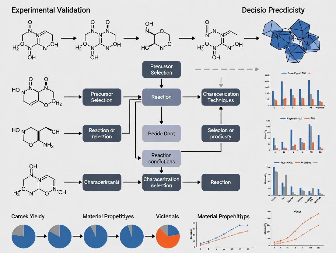
Experimental Validation Workflow

The following diagram outlines a robust workflow for experimentally validating synthesizability predictions, integrating both computational and lab-based steps.

This table details essential computational and experimental resources for conducting synthesizability research.

Item Name	Function / Purpose	Key Considerations
Retrosynthesis Software (e.g., AiZynthFinder, IBM RXN) [3]	Predicts synthetic pathways for a target molecule.	Check the scope of the built-in reaction template library and building block database.
Synthesizability LLMs (e.g., CSLLM) [1]	Directly predicts the synthesizability of crystal structures and suggests precursors.	Requires a text-based representation of the crystal structure (e.g., CIF, POSCAR).
Commercial Building Block Libraries (e.g., Enamine, Sigma-Aldrich)	Source of starting materials for proposed synthetic routes.	Prioritize readily available and affordable reagents to increase practical feasibility [3].
Heuristic Scoring Tools (e.g., SA Score, SYBA) [3]	Provides a fast, initial complexity estimate for molecules.	Use for initial triage, not as a definitive synthesizability metric. Can be well-correlated with retrosynthesis in drug-like space [3].
High-Throughput Experimentation (HTE) Rigs	Allows for rapid, parallel experimental testing of multiple synthetic conditions or precursors.	Essential for efficiently validating predictions for a large set of candidate materials [2].

Troubleshooting Guide: Synthesizability Predictions

FAQ: Addressing Common Experimental-Simulation Gaps

Q1: My DFT simulations show a candidate material is stable on the convex hull (Ehull = 0), but repeated synthesis attempts fail. Why? This common issue arises because the Energy Above Hull is a thermodynamic metric calculated at 0 K, but real synthesis is governed by finite-temperature kinetics and pathways.

• Troubleshooting Steps:
  • Investigate Kinetic Barriers: A zero Ehull confirms thermodynamic stability but does not guarantee a viable kinetic pathway for formation. The material may be trapped in a metastable state.
  • Check Phase Competition: Examine if your target phase decomposes into other polymorphs or compounds under your synthesis conditions. The existence of multiple polymorphs with similar energies complicates selective synthesis [2].
  • Validate Synthesis Parameters: Recalculate the Ehull using functionals that account for entropic contributions or finite-temperature effects, if computationally feasible. Experimentally, consider alternative synthesis routes like chemical vapor transport or flux methods that can lower kinetic barriers.

Q2: I am screening a ternary oxide, and the charge-balancing rule flags it as "forbidden," yet I found a published paper reporting its synthesis. Is the filter wrong? Yes, the rigid charge-balancing filter can produce false negatives. It is an imperfect proxy because it cannot account for different bonding environments, such as metallic or covalent character, which allow for non-integer oxidation states and charge transfer [4].

• Troubleshooting Steps:
  • Quantify Filter Reliability: Recognize that charge-balancing alone is a weak predictor. One study found only 37% of synthesized inorganic materials in a database were charge-balanced according to common oxidation states [4].
  • Use Complementary Filters: Augment the charge neutrality check with other human-knowledge filters, such as electronegativity balance or stoichiometric variation analysis [5].
  • Employ a Data-Driven Model: Use a machine learning-based synthesizability model (e.g., SynthNN) that learns the complex relationships between composition, structure, and synthesizability from all known materials, going beyond rigid rules [4].

Q3: How reliable is a slightly positive Energy Above Hull (e.g., 50 meV/atom) as a synthesizability filter? The reliability of a positive Ehull is highly system-dependent. While a high Ehull (e.g., > 200 meV/atom) generally indicates instability, many metastable materials with low positive Ehull are synthesizable.

• Troubleshooting Steps:
  • Consult Experimental Databases: Search the ICSD and literature for analogous materials. If known metastable phases (e.g., diamond, martensite) exist in similar chemical systems, your candidate might be synthesizable [6].
  • Consider Synthesis-Derived Stabilization: Materials can be stabilized by kinetics, entropy, or specific synthesis conditions not captured by DFT. High-pressure or low-temperature synthesis can access metastable phases [6].
  • Use a Probabilistic Framework: Instead of a hard Ehull cutoff, use a machine learning model that outputs a synthesizability score (SC). One such model reported an 82.6% precision in identifying synthesizable ternary crystals, which is often more accurate than an Ehull threshold [2].

Table 1: Performance Comparison of Common Synthesizability Proxies

Proxy Metric	Underlying Principle	Key Quantitative Limitation	Reported Performance
Charge Balancing	Chemical intuition (ionic charge neutrality)	Inflexible; ignores covalent/metallic bonding [4].	Only 37% of known synthesized inorganic materials are charge-balanced [4].
Energy Above Hull (Ehull)	Thermodynamic stability at 0 K	Fails to account for kinetics, entropy, and finite-temperature effects [7] [6].	Captures only ~50% of synthesized inorganic materials [4].
Machine Learning (SynthNN)	Data-driven patterns from all known materials	Requires large, clean datasets; can be a "black box." [4]	1.5x higher precision than human experts and completes tasks much faster [4].

Table 2: A Toolkit for Experimental Validation of Synthesizability Predictions

Tool / Reagent	Function in Validating Synthesizability
High-Throughput Automated Laboratory	Executes synthesis recipes from computational planning at scale, enabling rapid experimental feedback on dozens of candidates [7].
Literature-Mined Synthesis Data	Provides real-world reaction conditions (precursors, temperature) to ground-truth computational predictions and plan feasible experiments [7] [6].
Human-Curated Dataset (e.g., Ternary Oxides)	Offers a high-quality, reliable benchmark for evaluating and improving both computational filters and data-driven models, as text-mined data can have low accuracy [6].
Retrosynthesis Models (e.g., AiZynthFinder)	For molecular materials, these models propose viable synthetic routes, offering a more nuanced assessement of synthetic accessibility than simple scores [8].

Detailed Experimental Protocols for Validation

Protocol 1: Validating with a Human-Curated Solid-State Synthesis Dataset

This protocol uses high-quality, manually extracted data to assess the false positive/negative rate of your synthesizability filters [6].

• Data Curation:

  • Source a list of candidate compositions from your computational pipeline.
  • Manually extract synthesis information from the literature for these compositions using resources like the ICSD, Web of Science, and Google Scholar.
  • For each composition, label it as "solid-state synthesized" if a solid-state synthesis is reported, or "non-solid-state synthesized" if it was made by other methods (e.g., sol-gel, flux). Record details like highest heating temperature, atmosphere, and precursors.

• Model Benchmarking:

  • Apply your computational proxies (e.g., Ehull threshold, charge-balancing) to the curated list of compositions.
  • Compare the predictions against the manual labels to calculate precision, recall, and identify specific failure cases (e.g., compounds that are synthesizable but violate charge neutrality).

• PU Learning Application:

  • Use the reliable "solid-state synthesized" data as positive labels.
  • Treat a large set of hypothetical compositions from databases like the Materials Project as unlabeled data.
  • Train a Positive-Unlabeled (PU) learning model to probabilistically identify synthesizable materials from the unlabeled set, providing a data-driven prioritization list [6].

Protocol 2: High-Throughput Experimental Feedback Loop

This protocol, derived from state-of-the-art research, closes the loop between prediction and experimental validation [7].

• Candidate Prioritization:

  • Screen a large pool of computational structures (e.g., from the Materials Project, GNoME) using an ensemble synthesizability score that combines both compositional and structural models.
  • Rank candidates using a rank-average ensemble and apply practical filters (e.g., excluding toxic or rare elements).

• Synthesis Planning:

  • For the top-ranked candidates, use a precursor-suggestion model (e.g., Retro-Rank-In) to generate a list of viable solid-state precursors.
  • Employ a synthesis condition model (e.g., SyntMTE) to predict the calcination temperature required to form the target phase. Balance the reaction and compute precursor quantities.

• Automated Synthesis & Characterization:

  • Execute the synthesis recipes in a high-throughput automated laboratory.
  • Characterize the resulting products using X-ray diffraction (XRD).
  • Compare the experimental XRD pattern to the computationally predicted pattern of the target structure to confirm successful synthesis. This process has been shown to successfully synthesize target materials, including novel ones, within days [7].

Protocol 3: Integrating Retrosynthesis Tools for Molecular Materials

For organic molecules or metal-organic frameworks, synthesizability is often assessed by the existence of a plausible synthetic route [8].

• Route Solving:

  • Input the SMILES string of your target molecule into a retrosynthesis tool (e.g., AiZynthFinder, SYNTHIA).
  • Configure the tool to use a library of available building blocks and reaction templates.
  • Run the search to determine if the tool can find one or more viable routes to the target molecule.

• Synthesizability Optimization:

  • In generative molecular design, directly integrate the retrosynthesis tool's output (e.g., a binary "solved/not solved" flag or a score) into the multi-parameter optimization objective.
  • This guides the generative model to propose structures that are not only optimal in terms of properties (e.g., binding affinity) but also have a higher likelihood of being synthesizable, as deemed by the retrosynthesis model [8].

Workflow Visualization: From Prediction to Validation

Validating Synthesizability Predictions Workflow

FAQs: Predictive Models and Experimental Validation

What are the fundamental types of predictive models used in research?

Predictive models can be broadly categorized into several types, each suited for different kinds of data and research questions [9]:

• Classification Models: These models place data into specific categories (e.g., yes/no) based on historical data. They are ideal for answering discrete questions, such as "Is this transaction fraudulent?" or "Will this patient respond to the treatment?" [9].
• Clustering Models: These models sort data into separate, nested groups based on similar attributes without pre-defined categories. This is useful for patient stratification or identifying patterns in molecular profiles [9] [10].
• Forecast Models: These are among the most widely used models and deal with metric value prediction. They estimate numerical values for new data based on historical data, such as predicting inventory needs or the volume of experimental results [9].
• Outliers Models: These models are designed to identify anomalous data entries within a dataset. They are critical for detecting fraud, experimental errors, or unusual biological responses [9].
• Time Series Models: This type involves a sequence of data points collected over time. It uses historical data to forecast future values, considering trends and seasonal variations, which is useful for monitoring tumor progression or long-term experimental outcomes [9] [10].

How do I validate a predictive model to ensure its results are reliable for my research?

Proper validation is critical to ensure your predictive model is robust and not overfitted to your initial dataset. Key strategies include [11] [12]:

• Data Splitting: Partition your dataset into a training set (to build the model) and a testing set (to evaluate its performance). The split should be random, and both datasets must be representative of the actual population. A third validation dataset is often used to provide an unbiased evaluation of the final model and to tune model parameters [12].
• Cross-Validation: This technique, such as k-fold cross-validation, repeatedly partitions the data into different training and test sets. It helps ensure that your model's performance is consistent and not dependent on a single, potentially lucky, data split [11] [12].
• Comparison with Experimental Data: For research validation, directly compare the model's predictions against results from experimental models. In oncology, for instance, this involves cross-validating AI predictions with data from patient-derived xenografts (PDXs), organoids, or tumoroids to ensure biological relevance [10].
• Managing Bias and Variance: Strive to balance bias (error from erroneous assumptions) and variance (error from sensitivity to small fluctuations in the training set). A good model should have low bias and low variance [12].

What are common pitfalls when training predictive models, and how can I troubleshoot them?

Researchers often encounter several specific issues during model development. The table below outlines common problems and their solutions.

Problem	Description	Troubleshooting Steps
Overfitting	Model performs well on training data but poorly on unseen test data. It has essentially "memorized" the noise in the training set.	- Simplify the model by reducing the number of parameters [9].- Apply cross-validation to get a better estimate of real-world performance [11] [12].- Increase the size of your training dataset if possible [10].
Data Imbalance	The dataset has very few examples of one class (e.g., active compounds) compared to another (inactive compounds), biasing the model toward the majority class [13].	- Use resampling techniques (oversampling the minority class or undersampling the majority class) [13].- Utilize algorithms like Random Forest that are relatively resistant to overfitting and can handle imbalance [9].- Employ appropriate evaluation metrics like F1-score instead of just accuracy [9].
Model Interpretability ("Black Box")	It is difficult to understand how a complex model (e.g., deep neural network) arrived at a specific prediction, which is a significant hurdle for scientific acceptance [10].	- Use Explainable AI (XAI) techniques to interpret model decisions [10].- Perform feature importance analysis to identify which input variables had the most significant impact on the prediction [10].- Consider using inherently more interpretable models like Generalized Linear Models (GLMs) or decision trees where appropriate [9].
Insufficient or Low-Quality Data	The model's performance is limited by a small dataset, missing values, or high experimental error in the training data [14] [10].	- Perform rigorous data preprocessing: handle missing values, normalize data, and remove outliers [9].- Engage domain experts to guide data curation and feature engineering [9] [12].- Leverage data from public repositories and biobanks to augment your dataset [10].

How are Large Language Models (LLMs) like GPT-4 being applied in predictive tasks within materials science and drug discovery?

LLMs are moving beyond text generation to become powerful tools for scientific prediction. Key applications include [13]:

• Intelligent Data Extraction: LLMs can mine vast scientific literature to extract valuable, unstructured information such as synthesis conditions and material properties, creating structured, queryable databases for downstream predictive modeling [13].
• Predicting Synthesis Conditions: Fine-tuned LLMs can act as "recommender" tools, predicting feasible synthesis conditions for novel materials based on textual descriptions of their precursors or composition [13].
• Learning Structure-Property Relationships: By training on comprehensive datasets of chemical information, LLMs can learn the complex relationships between a material's structure and its properties. For example, they can achieve high accuracy in predicting hydrogen storage performance or synthesisability from rich text descriptions of atomic-level structures [13].
• Multi-Agent Experimental Systems: The most advanced applications use an LLM as a central "brain" to coordinate research workflows. These systems can plan multi-step procedures, interface with simulation tools, and even operate robotic platforms for automated experimentation [13].

The following diagram illustrates a typical workflow for using and validating an LLM for synthesizability predictions.

What experimental protocols are used to validate AI-driven predictions in oncology research?

In fields like oncology, computational predictions must be rigorously validated through biological experiments. A standard protocol involves these key methodologies [10]:

• Cross-Validation with Patient-Derived Models:

  • Purpose: To compare AI predictions against biological responses in models that closely mimic human disease.
  • Methodology: Predictions of drug efficacy or tumor behavior are tested in vitro and in vivo using Patient-Derived Xenografts (PDXs), organoids, and tumoroids. For example, a model predicting the response to a targeted therapy is validated against the actual response observed in a PDX model carrying the same genetic mutation [10].

• Longitudinal Data Integration for Model Refinement:

  • Purpose: To improve the predictive accuracy of AI algorithms over time by incorporating dynamic, time-series data.
  • Methodology: Time-series data from experimental studies, such as tumor growth trajectories from PDX models, is fed back into the AI system. This data is used to retrain and refine the predictive models, ensuring they better reflect real-world biological dynamics [10].

• Multi-Omics Data Fusion for Enhanced Prediction:

  • Purpose: To capture the complexity of tumor biology by integrating diverse biological datasets.
  • Methodology: AI platforms unify data from genomics (mutations), transcriptomics (gene expression), and proteomics (protein interactions). This integrated dataset is used to build and validate models, ensuring predictions account for the multi-faceted nature of cancer [10]. For instance, this approach can identify novel biomarkers that are subsequently validated in clinical studies [10].

The workflow for this validation process is outlined below.

The Scientist's Toolkit: Research Reagent Solutions

This table details key materials and computational tools used in developing and validating predictive models for drug discovery and materials science.

Item	Function
Patient-Derived Xenografts (PDXs)	In vivo models where human tumor tissue is implanted into immunodeficient mice. They are a gold standard for validating predictions of drug efficacy and tumor behavior as they retain the genetic and histological characteristics of the original patient tumor [10].
Organoids & Tumoroids	3D in vitro cell cultures that self-organize into structures mimicking organs or tumors. They are used for medium-throughput validation of drug responses and for studying biological mechanisms in a controlled environment [10].
Multi-Omics Datasets	Integrated datasets comprising genomics, transcriptomics, proteomics, and metabolomics. They are used to train AI models and provide a holistic view of tumor biology, enabling more accurate predictions of therapeutic outcomes [10].
Random Forest Algorithm	A popular machine learning algorithm capable of both classification and regression. It is accurate, efficient with large databases, resistant to overfitting, and can estimate which variables are important in classification [9].
Generalized Linear Model (GLM)	A flexible generalization of linear regression that allows for response variables with non-normal distributions. It trains quickly, is relatively straightforward to interpret, and provides a clear understanding of predictor influence [9].
Open-Source LLMs (e.g., Llama, Qwen)	Large language models with publicly available weights and architectures. They offer an alternative to closed-source models, providing greater transparency, reproducibility, cost-effectiveness, and data privacy for scientific tasks like data extraction and prediction [13].
Dipropyldiphosphonic acid	Dipropyldiphosphonic acid, CAS:71760-04-8, MF:C6H16O5P2, MW:230.14 g/mol
Decanoic acid, 6-hydroxy-	Decanoic acid, 6-hydroxy-, CAS:16899-10-8, MF:C10H20O3, MW:188.26 g/mol

The Critical Need for Experimental Validation in the Discovery Workflow

FAQs on Synthesizability Prediction and Validation

Q1: What is the difference between thermodynamic stability and synthesizability? Thermodynamic stability, often assessed via formation energy or energy above the convex hull (Ehull), is a traditional but insufficient proxy for synthesizability. Many metastable structures (with less favorable formation energies) are successfully synthesized, while numerous structures with favorable formation energies remain unsynthesized. Synthesizability is a more complex property influenced by kinetic factors, precursor availability, and specific reaction conditions [1] [2].

Q2: Why is experimental validation crucial for computational synthesizability predictions? Computational models, while powerful, require experimental "reality checks." Validation confirms that the proposed method is practically useful and that the claims put forth are correct. Without it, claims that a newly generated material or molecule has better performance are difficult to substantiate [15].

Q3: A model predicted my compound is synthesizable, but my experiments are failing. What could be wrong? This is a common challenge. The issue often lies in the transfer from general synthesizability to your specific lab context.

• Precursor Availability: The prediction might assume an infinite supply of building blocks, while your in-house resources are limited. Re-run synthesis planning with your specific available precursors [16].
• Synthetic Method: The predicted synthetic route (e.g., solid-state vs. solution) may not be optimal for your compound. Verify that the suggested method aligns with the material's properties [1].
• Reaction Kinetics: While the reaction may be thermodynamically feasible, kinetic barriers could be preventing it. Investigate alternative reaction conditions like temperature, pressure, or catalysts.

Q4: How can I adapt general synthesizability predictions to my laboratory's specific available resources? You can develop a rapidly retrainable, in-house synthesizability score. This involves using Computer-Aided Synthesis Planning (CASP) tools configured with your specific inventory of building blocks to generate training data. A model trained on this data can then accurately predict whether a molecule is synthesizable with your in-house resources [16].

Troubleshooting Guide: Experimental Validation

Problem Area	Possible Cause	Investigation & Action
Failed Synthesis	Incorrect or unavailable precursors.	Verify precursor stability and purity; use CASP with your building block inventory to find viable alternatives [1] [16].
	Synthetic method misalignment.	Re-evaluate the recommended method (e.g., solid-state, solution); consult literature for analogous compounds [1].
	Unfavorable reaction kinetics.	Systematically vary reaction conditions (temperature, time, pressure) to overcome kinetic barriers.
Impure Product	Side reactions or incomplete conversion.	Analyze byproducts; optimize reaction stoichiometry and purification protocols (e.g., recrystallization, chromatography).
Property Mismatch	Incorrect crystal structure or phase.	Use characterization (XRD, NMR) to confirm the synthesized structure matches the predicted one; check for polymorphs [15].

Quantitative Comparison of Synthesizability Assessment Methods

The table below summarizes different approaches to evaluating synthesizability, highlighting the performance of modern machine learning methods.

Assessment Method	Key Metric	Reported Performance / Limitation	Key Principle
Thermodynamic Stability [1] [2]	Energy above hull (Ehull)	~74.1% accuracy; insufficient as many metastable structures are synthesizable.	Assumes thermodynamic stability implies synthesizability.
Kinetic Stability [1]	Phonon spectrum (lowest frequency)	~82.2% accuracy; structures with imaginary frequencies can be synthesized.	Assesses dynamic stability against small displacements.
Crystal-likeness Score (CLscore) [2]	ML-based score	86.2% recall for synthesized materials; used to filter non-synthesizable structures.	Machine learning model trained on existing crystal data.
Synthesizability Score (SC) [2]	ML-based classification	82.6% precision, 80.6% recall for ternary crystals.	Fourier-transformed crystal properties with a deep learning classifier.
Crystal Synthesis LLM (CSLLM) [1]	LLM-based classification	98.6% accuracy; demonstrates high generalization to complex structures.	Large language model fine-tuned on a comprehensive dataset of crystal structures.

Experimental Protocols for Validation

Protocol 1: Validating Solid-State Synthesis from Computational Predictions

This protocol provides a general workflow for experimentally validating the synthesizability of a predicted inorganic crystal structure.

1. Precursor Preparation:

• Based on the Precursor LLM output or CASP suggestion, identify solid-state precursors (e.g., metal oxides, carbonates).
• Weigh precursors according to the stoichiometry of the target compound.
• Use a mortar and pestle or a ball mill to mix and grind the precursors thoroughly to ensure homogeneity and increase surface area for reaction.

2. Initial Heat Treatment:

• Place the mixed powder in a high-temperature crucible (e.g., alumina, platinum).
• Insert the crucible into a box furnace or tube furnace.
• Heat the sample at a moderate rate (e.g., 5-10°C per minute) to a target temperature below the final sintering temperature for calcination. This step decomposes carbonates or nitrates and initiates solid-state diffusion.
• After calcination, allow the furnace to cool naturally. Re-grind the powder to ensure homogeneity.

3. Final Sintering and Phase Formation:

• Press the calcined powder into pellets using a hydraulic press to improve inter-particle contact.
• Sinter the pellets at the final, higher temperature (determined from literature or phase diagrams) for an extended period (e.g., 12-48 hours) to facilitate complete reaction and crystal growth.

4. Product Characterization:

• X-ray Diffraction (XRD): Grind a portion of the sintered pellet and analyze its powder XRD pattern. Compare the measured pattern to the computationally predicted crystal structure to confirm successful synthesis and phase purity.
• Additional Techniques: Use techniques like Scanning Electron Microscopy (SEM) for morphology and Energy-Dispersive X-ray Spectroscopy (EDS) for elemental composition analysis.

Protocol 2: Computer-Aided Synthesis Planning (CASP) for Small Molecules

This protocol outlines using CASP to plan and validate the synthesis of small organic molecules.

1. Input the Target Molecule:

• Provide the structure of the target molecule in a standard format (e.g., SMILES) to a CASP tool (e.g., AiZynthFinder).

2. Configure Building Block Settings:

• For general synthesizability, use a large commercial building block database (e.g., Zinc, ~17.4 million compounds).
• For in-house synthesizability, configure the tool to use your specific, limited inventory of available building blocks (e.g., 6,000 compounds) [16].

3. Execute Retrosynthetic Analysis:

• Run the CASP algorithm. It will recursively deconstruct the target molecule into simpler precursors until it identifies a pathway to your available building blocks.
• Note that using a limited in-house inventory may result in synthesis routes that are, on average, two steps longer than those using a full commercial database [16].

4. Evaluate and Select a Synthesis Route:

• Review the proposed routes based on the number of steps, predicted yields, and the familiarity/reliability of the suggested reactions.
• Use this CASP-generated route as a guide for laboratory synthesis.

The Scientist's Toolkit: Key Research Reagents & Materials

Item	Function in Validation
Solid-State Precursors	High-purity powders (e.g., metal oxides, carbonates) that react to form the target inorganic crystal material [1].
Molecular Building Blocks	Commercially available or in-house stockpiled organic molecules used as starting materials in CASP-planned syntheses [16].
CASP Software	Computer-aided synthesis planning tools that deconstruct target molecules into viable synthesis routes using available building blocks [16].
Inorganic Crystal Structure Database (ICSD)	A curated database of experimentally synthesized crystal structures, used as a source of ground-truth data for training and validating synthesizability models [1] [2].
(S,R,R,R)-Orlistat	(S,R,R,R)-Orlistat
Glutathione sulfinanilide	Glutathione sulfinanilide, MF:C16H22N4O7S, MW:414.4 g/mol

Experimental Validation Workflow

The diagram below illustrates a robust, iterative workflow for validating computational synthesizability predictions through experimentation.

Integrating Prediction with Experimental Validation

This diagram outlines the full discovery pipeline, from initial computational design to experimental validation and model refinement.

A Blueprint for Experimental Validation: From Candidate Selection to Synthesis

FAQs: Core Concepts of Synthesizability and Screening

Q1: What is a synthesizability score, and why is it crucial for my research? A synthesizability score is a computational prediction of the likelihood that a proposed molecular or material structure can be successfully synthesized in a laboratory. It is crucial because it bridges the gap between in-silico design and real-world experimental validation. Relying solely on stable, low-energy structures from simulations like Density Functional Theory (DFT) often leads to candidates that are not experimentally accessible, as these calculations can overlook finite-temperature effects and kinetic factors [7]. Using a synthesizability score helps prioritize candidates that are not just theoretically stable, but also practically makeable, saving significant time and resources [17].

Q2: What is the difference between general and in-house synthesizability? The key difference lies in the availability of building blocks or precursors:

• General Synthesizability assumes a near-infinite supply of commercially available building blocks (e.g., from databases like Zinc with 17.4 million compounds) [18].
• In-House Synthesizability is tailored to a specific laboratory's limited, available stock of building blocks (e.g., 6,000 compounds). This reflects the real-world constraints of a research environment. While using an in-house set may result in synthesis routes that are, on average, two reaction steps longer, the drop in overall synthesis planning success can be as low as -12% compared to a vast commercial library [18].

Q3: What is rank-based screening, and how is it better than using a fixed threshold? Rank-based screening is a method for ordering a large pool of candidate molecules or materials based on their synthesizability scores and other desired properties. Instead of applying a fixed probability cutoff (e.g., >0.8), candidates are ranked relative to each other. A powerful method is the rank-average ensemble (or Borda fusion), which combines rankings from multiple models [7]. This method is superior to a fixed threshold because it provides a relative measure of synthesizability within your specific candidate pool, ensuring you select the most promising candidates for your particular project, even if absolute probabilities are low.

Q4: My top-ranked candidate failed synthesis. What are the most likely reasons? Several factors can lead to this discrepancy:

• Gaps in Training Data: The synthesizability model may not have been trained on data representative of your specific chemical space or synthesis conditions [7].
• Precursor Impurities or Availability: The suggested synthesis route might rely on precursors that are impure, unavailable, or unstable in your lab [18].
• Kinetic vs. Thermodynamic Control: The model may predict thermodynamic stability, but the synthesis might be kinetically hindered, requiring specific reaction conditions not captured by the plan [7].
• In-House Building Block Mismatch: The general synthesizability score might have ranked the candidate highly, but your specific in-house building block collection may not allow for an efficient route, leading to failure or impure products [18].

Troubleshooting Guides

Problem 1: Low Success Rate in Synthesis Planning (CASP) with In-House Building Blocks

• Symptoms: Computer-Aided Synthesis Planning (CASP) tools fail to find routes for a high percentage of your candidate molecules when configured with your lab's building block list.
• Investigation Steps:
  • Benchmark Your Setup: Test your CASP tool on a standard dataset (e.g., a drug-like ChEMBL subset) using both your in-house blocks and a large commercial library. A performance drop of around 12% is expected; a larger gap indicates an issue [18].
  • Analyze Building Block Diversity: Check if your in-house collection lacks diversity in key chemical regions needed for your target candidates.
• Resolution Steps:
  • Retrain a Custom Synthesizability Score: Train a rapid, CASP-based synthesizability score specifically on your in-house building blocks. A well-chosen dataset of 10,000 molecules can be sufficient for effective retraining, capturing your lab's specific synthesizability context without high computational cost [18].
  • Strategic Building Block Acquisition: Use the failed candidates to identify frequently missing precursor structures and make targeted purchases to expand your in-house library.

Problem 2: Disagreement Between Synthesizability Score and Synthesis Planning

• Symptoms: A candidate receives a high synthesizability score from a learned model, but the CASP tool cannot find a synthesis route (or vice versa).
• Investigation Steps:
  • Interrogate the Score's Basis: Determine if the score is compositional, structural, or CASP-based. A composition-only model might miss complex structural synthesis barriers [7].
  • Check CASP Parameters: Review the synthesis planning configuration, including the maximum number of reaction steps and the allowed reaction types. Overly restrictive settings can cause false negatives.
• Resolution Steps:
  • Implement a Rank-Average Ensemble: Combine the strengths of different models. Use both a general/compositional score and a CASP-based score, then aggregate their outputs using a rank-average to create a more robust priority list [7].
  • Manual Route Inspection: For critical high-score candidates that CASP fails on, engage an experienced medicinal chemist to manually evaluate potential retrosynthetic pathways that the AI might have missed.

Problem 3: Successfully Synthesized Compound Lacks Desired Activity

• Symptoms: A candidate, ranked highly for both synthesizability and predicted activity (e.g., via a QSAR model), is successfully made but shows no biochemical efficacy in testing.
• Investigation Steps:
  • Verify Compound Purity and Structure: Confirm via analytical methods (e.g., NMR, LC-MS) that the synthesized compound is the intended structure and is pure.
  • Re-evaluate the Activity Model: Scrutinize the predictive model used for the biological activity. Was it trained on sufficiently diverse and relevant data? Does the candidate fall outside the model's applicability domain?
• Resolution Steps:
  • Adopt Multi-Objective Optimization: Integrate synthesizability and activity predictions into a unified, multi-objective de novo design workflow. This ensures the generative AI creates structures that balance both synthesizability and potency from the outset, rather than just filtering for them post-generation [18].
  • Analyze the Broader Candidate Space: Examine other highly-ranked candidates from your generation run. They may reveal alternative, active scaffolds with similar synthesizability that can provide new ligand ideas for your target [18].

Experimental Protocols & Data

Table 1: Quantitative Comparison of Synthesis Planning Performance

This table summarizes the performance of synthesis planning when using a large commercial building block library versus a limited in-house collection, adapted from a real-world case study [18].

Building Block Set	Number of Building Blocks	Solvability Rate (Caspyrus Centroids)	Average Shortest Synthesis Route (Steps)
Commercial (Zinc)	17.4 million	~70%	Shorter by ~2 steps
In-House (Led3)	5,955	~60%	Longer by ~2 steps

Table 2: Key Research Reagent Solutions for Validating Synthesizability

Item	Function in Experiment
Computer-Aided Synthesis Planning (CASP) Tool (e.g., AiZynthFinder)	An open-source toolkit that performs retrosynthetic analysis to deconstruct target molecules into available building blocks and proposes viable synthesis routes [18].
In-House Building Block Collection	A curated, digitally cataloged inventory of chemical precursors physically available in your laboratory. This is the fundamental constraint for defining in-house synthesizability [18].
Synthesizability Prediction Model	A machine learning model (e.g., a graph neural network for structures, transformer for compositions) that outputs a score estimating synthesis probability. An ensemble model combining both is state-of-the-art [7].
High-Throughput Synthesis Laboratory	An automated lab setup (e.g., with a robotic muffle furnace) that allows for the parallel synthesis of multiple candidates based on AI-predicted recipes, drastically speeding up validation [7].
Characterization Equipment (e.g., XRD)	X-ray Diffraction is used to verify that the synthesized product's crystal structure matches the computationally predicted target structure [7].

Protocol: Experimental Validation of Synthesizability Predictions

This protocol outlines the key steps for a synthesizability-guided discovery pipeline, integrating elements from both drug and materials discovery [18] [7].

• Candidate Pool Generation: Start with a large, computationally generated pool of candidate molecules or materials (e.g., from a de novo design algorithm or a massive database like GNoME).
• Synthesizability Scoring & Ranking:
  • Apply your synthesizability model(s) to the entire candidate pool.
  • Use a rank-average ensemble to combine scores from different models (e.g., compositional and structural) into a single, robust ranking.
  • Apply filters (e.g., exclude toxic elements, focus on oxides) to narrow the list to a few hundred high-priority candidates.
• Synthesis Planning: For the top-ranked candidates, use a CASP tool to generate specific synthesis routes using your in-house or readily available building blocks.
• Experimental Synthesis: Execute the suggested synthesis routes in the lab. A high-throughput, automated platform is ideal for testing multiple candidates in parallel.
• Characterization & Validation: Analyze the synthesized products using techniques like XRD, NMR, or mass spectrometry to confirm the identity and purity of the target compound.
• Feedback Loop: Use the experimental results (successes and failures) to retrain and improve your synthesizability models, creating a continuous learning cycle.

Workflow Visualization

Diagram 1: Synthesizability-Guided Validation Workflow

Diagram 2: Architecture of a Unified Synthesizability Model

This diagram details the architecture of a state-of-the-art synthesizability model that integrates both compositional and structural information [7].

This technical support guide outlines the experimental validation of a computational pipeline designed for the rapid identification and synthesis of structural analogs of known drugs [19] [20]. The overarching thesis of this research is to bridge the gap between in silico predictions of synthesizability and experimental confirmation, thereby accelerating drug development [21]. The process involves several key stages: diversification of a parent molecule to create analogs, retrosynthetic analysis to identify substrates, forward-synthesis guided towards the parent, and finally, experimental evaluation of binding affinity and medicinal-chemical properties [20].

The following FAQs, troubleshooting guides, and protocols are designed to support researchers in experimentally validating such computational predictions, using the documented case studies of Ketoprofen and Donepezil analogs as a foundation [19].

Frequently Asked Questions (FAQs) & Troubleshooting

FAQ 1: The synthesis of my computer-designed analog failed. What are the primary causes? Synthesis failure can often be attributed to the accuracy of the initial retrosynthetic analysis.

• Cause: The retrosynthetic algorithm may have suggested a disconnection that is theoretically valid but practically low-yielding or incompatible with other functional groups in the molecule.
• Solution: Re-evaluate the proposed route manually. Consider using alternative starting materials identified through the "replica" method, where substructure replacements are made to the parent before retrosynthesis to ensure starting materials retain mutual reactivity [20]. Furthermore, employ a synthetic feasibility score (e.g., FSscore) that can be fine-tuned with human expert feedback to rank the synthesizability of proposed analogs before committing to experimental work [22].

FAQ 2: My compound showed poor binding affinity despite favorable computational docking. Why? This is a common challenge, as binding affinity predictions may only be accurate to within an order of magnitude [19] [20].

• Cause: Docking programs primarily predict the binding mode and provide a rough estimate of affinity. They may struggle to accurately calculate solvation effects, entropy, or subtle protein flexibility [20].
• Solution: Use docking scores as a tool for initial prioritization and to discern promising binders from inadequate ones, but do not rely on them to discriminate between moderate (μM) and high-affinity (nM) binders. Always plan for experimental validation [19]. Ensure your docking protocol includes multiple runs and cross-validation with different software where possible.

FAQ 3: I am observing high background noise or non-specific binding (NSB) in my binding assay (e.g., ELISA). What should I check? High background is frequently caused by contamination or improper washing [23].

• Causes and Solutions:
  • Contamination: The assays are extremely sensitive. Avoid performing assays in areas where concentrated forms of the analyte (e.g., cell culture media, sera) are handled. Use dedicated, clean pipettes and aerosol barrier tips. Do not use plate washers that have been previously exposed to concentrated analyte solutions [23].
  • Incomplete Washing: Ensure the microtiter wells are washed thoroughly according to the kit's protocol. Incomplete washing can lead to carryover of unbound reagent [23].
  • Reagent Contamination: If using an alkaline phosphatase-based system (e.g., with PNPP substrate), environmental contaminants can cause high background. Only withdraw the substrate needed for the immediate assay and do not return unused portions to the stock bottle [23].

FAQ 4: My dose-response curve has a poor fit, making IC50/EC50 determination unreliable. How can I improve data analysis? The choice of curve-fitting algorithm is critical for immunoassays and binding data [23].

• Solution: Avoid using simple linear regression, as most bioassays are inherently non-linear. Instead, use robust fitting routines such as Point-to-Point, Cubic Spline, or 4-Parameter Logistic (4PL) regression [23]. To validate your chosen method, "back-fit" your standard curve data as unknowns; the algorithm should recover the nominal values of the standards accurately.

FAQ 5: How can I assess the robustness of my bioassay beyond the size of the assay window? The Z'-factor is a key metric that considers both the assay window and the data variability [24].

• Implementation: The Z'-factor is calculated using the formula: Z' = 1 - [ (3 * SD_high + 3 * SD_low) / |Mean_high - Mean_low| ] where SD_high and SD_low are the standard deviations of the high (e.g., maximum signal) and low (e.g., minimum signal) controls, and Mean_high and Mean_low are their respective mean signals. A Z'-factor > 0.5 is generally considered indicative of a robust assay suitable for screening [24].

Quantitative Data from Validated Case Studies

The following tables summarize the key experimental outcomes from the referenced study, providing a benchmark for successful validation.

Table 1: Experimental Validation of Computer-Designed Syntheses

Parent Drug	Number of Analogs Proposed for Synthesis	Number of Successful Syntheses	Synthesis Success Rate
Ketoprofen	7	7	100%
Donepezil	6	5	83%
Total	13	12	92%

Table 2: Experimental Binding Affinity of Validated Analogs

Parent Drug	Target Protein	Parent Drug Binding Affinity	Best Analog Binding Affinity	Potency of Best Analog vs. Parent
Ketoprofen	COX-2	0.69 μM	0.61 μM	Slightly more potent
Donepezil	Acetylcholinesterase (AChE)	21 nM	36 nM	Slightly less potent

Detailed Experimental Protocols

Protocol: Computational Analog Design and Synthesis Workflow

This protocol describes the core pipeline used to generate and validate the Ketoprofen and Donepezil analogs [20].

• Diversification: Start with the parent molecule. Perform in silico substructure replacements aimed at enhancing biological activity. These replacements can target peripheral groups or internal motifs (e.g., 1,3-disubstituted benzene rings, piperazines).
• Retrosynthetic Analysis: Subject the generated "replica" molecules to a retrosynthetic algorithm (e.g., Allchemy) to identify potential substrates.
• Substrate Curation: Augment the set of identified substrates with a small, static set of synthetically versatile "auxiliary" chemicals (e.g., NBS for bromination, bis(pinacolato)diboron for Suzuki couplings, mesyl chloride for activation) to enable a wider range of forward-synthesis reactions.
• Guided Forward-Synthesis:
  • Generation 0 (G0): Begin with the curated substrates.
  • Network Expansion: Apply a knowledge base of reaction transforms iteratively. To guide the network towards parent-like molecules, in each generation, retain only a pre-determined number (beam width, W) of products that are most structurally similar to the parent.
  • Cross-Generation Reactivity: After 1-2 generations, restrict reactions so that molecules in generation Gi can only react with species from earlier generations (G0 to Gi-1) to prevent combinatorial explosion.
• Synthesis Validation: Execute the top-ranked, computer-proposed synthetic routes in the laboratory using standard organic synthesis techniques.

Protocol: Measuring Binding Affinity via a TR-FRET Assay

This is a generalized protocol for binding assays, common in drug discovery [24].

• Plate Setup: Prepare a dilution series of the test compound in a low-volume, white assay plate. Include controls (high signal without inhibitor, low signal with a known potent inhibitor).
• Reaction Assembly:
  • Add the target protein (e.g., enzyme) to the wells.
  • Add the TR-FRET detection reagents. This typically includes a terbium (Tb)- or europium (Eu)-labeled donor antibody and a fluorescently-labeled acceptor tracer that binds to the target site.
• Incubation: Incubate the plate in the dark to allow the binding reaction to reach equilibrium.
• Reading the Plate: Use a compatible microplate reader with time-resolved (TR) detection and the correct emission filters. For a Tb donor, standard filters are 520 nm (acceptor) and 495 nm (donor).
• Data Analysis:
  • For each well, calculate the emission ratio (Acceptor Signal / Donor Signal).
  • Plot the emission ratio against the logarithm of the compound concentration.
  • Fit the data using a 4-parameter logistic model to determine the IC50 value.

Workflow Visualization

The following diagram illustrates the integrated computational and experimental workflow for validating structural analogs.

The Scientist's Toolkit: Key Research Reagents & Materials

Table 3: Essential Reagents for Analog Synthesis & Validation

Reagent / Material	Function / Application	Example / Notes
Synthetically Versatile Auxiliaries	Enables key reactions in forward-synthesis networks [20]	NBS (electrophilic halogenation), Bis(pinacolato)diboron (Suzuki coupling), Mesyl chloride (alcohol activation).
TR-FRET Detection Kit	Measures binding affinity in a homogeneous, high-throughput format [24]	Includes LanthaScreen Eu- or Tb-labeled donor and fluorescent acceptor tracer.
Assay-Specific Diluent	Diluting samples for binding assays without introducing matrix effects [23]	Formulated to match the standard curve matrix; prevents analyte adsorption and ensures accurate recovery.
Synthetic Feasibility Score (ML-based)	Computational prioritization of analogs based on predicted ease of synthesis [22]	e.g., FSscore; can be fine-tuned with expert feedback for specific chemical spaces (e.g., PROTACs, natural products).
Naveglitazar racemate	Naveglitazar Racemate
epi-Sesamin Monocatechol	epi-Sesamin Monocatechol, MF:C19H18O6, MW:342.3 g/mol	Chemical Reagent

The discovery of new inorganic crystals is a fundamental driver of innovation in energy storage, catalysis, and electronics. [25] Traditional materials discovery, reliant on experimentation and intuition, has long iteration cycles and limits the number of testable candidates. [25] High-throughput computational screening and generative models have dramatically accelerated the identification of promising hypothetical materials. [26] However, a significant challenge remains: bridging the gap between computational prediction and experimental realization. [27]

This case study establishes a technical support framework for researchers navigating this critical transition. It provides detailed protocols, troubleshooting guides, and resource information specifically designed to help validate the synthesizability of computationally predicted inorganic crystals, with a particular focus on materials generated by advanced models like MatterGen. [25] [28]

Computational Prediction: Frameworks and Validation

State-of-the-Art Generative Models

The field has moved beyond simple screening to the inverse design of materials using generative models. A leading model, MatterGen, is a diffusion-based generative model designed to create stable, diverse inorganic materials across the periodic table. [25]

Table 1: Performance Metrics of the MatterGen Generative Model for Crystal Prediction [25] [28]

Metric	Performance	Evaluation Context
Stability Rate	78% of generated structures	Energy within 0.1 eV/atom above the convex hull (Materials Project reference)
Structural Quality	95% of structures have RMSD < 0.076 Ã…	RMSD between generated and DFT-relaxed structures
Novelty & Diversity	61% of generated structures are new	Not matching any structure in the combined Alex-MP-ICSD dataset (850k+ structures)
Success Rate (SUN)	More than double previous models	Percentage of Stable, Unique, and New (SUN) materials generated

Validating Predictions Before Synthesis

Before committing to laboratory synthesis, a rigorous computational validation protocol is essential to prioritize the most promising candidates and avoid wasted resources.

Diagram 1: Computational validation workflow for predicted crystals.

The workflow involves several critical steps, each with a specific methodology:

• Initial Pre-screening with Machine Learning Force Fields (MLFFs): Universal Interatomic Potentials (UIPs) have advanced sufficiently to act as effective and cheap pre-filters for thermodynamic stability before running more computationally expensive Density Functional Theory (DFT) calculations. [27] This step rapidly eliminates clearly unstable configurations.

• DFT Relaxation and Stability Assessment: Candidates passing the initial screen undergo full relaxation using DFT, the computational workhorse of materials science. [27] [26] The key metric for stability is the energy above the convex hull, which quantifies a material's energetic competition with other phases in the same chemical system. A structure is typically considered potentially stable if this value is below 0.1 eV per atom. [25] [27] It is crucial to note that a low formation energy alone does not directly indicate thermodynamic stability; the convex hull distance is the more relevant metric. [27]

• Prototype Search and Novelty Check: Finally, stable predicted structures should be compared against extensive crystallographic databases (e.g., ICSD, Materials Project) using structure-matching algorithms to confirm their novelty. [25] This ensures that effort is not spent "re-discovering" known materials.

High-Throughput Synthesis and Experimental Validation

Synthesis Workflow for Novel Inorganics

Once a candidate is computationally validated, it proceeds to the laboratory synthesis phase. A generalized workflow for high-throughput synthesis is outlined below.

Diagram 2: High-throughput synthesis and validation loop.

The Scientist's Toolkit: Essential Research Reagents and Materials

A high-throughput synthesis lab requires specialized reagents and equipment to efficiently process and characterize multiple candidates.

Table 2: Essential Research Reagent Solutions for High-Throughput Synthesis

Item / Solution	Function / Purpose
High-Purity Elemental Precursors	Starting materials for solid-state reactions; purity is critical to avoid impurity phases.
Solvents (e.g., Water, Ethanol)	Medium for solution-based synthesis methods and precursor mixing.
Flux Agents (e.g., Molten Salts)	Lower synthesis temperature and improve crystal growth by providing a liquid medium.
Pellet Press Die	To form powdered precursors into dense pellets for solid-state reactions.
High-Temperature Furnaces	For annealing, sintering, and solid-state reactions (up to 1600°C+).
Controlled Atmosphere Glovebox	For handling air-sensitive precursors (e.g., alkali metals, sulfides).
Automated Liquid Handling Robots	To precisely dispense solution precursors for high-throughput experimentation.
ethanamine;phosphoric acid	ethanamine;phosphoric acid, CAS:60717-38-6, MF:C2H10NO4P, MW:143.08 g/mol
Ceftiofur Thiolactone	Ceftiofur Thiolactone CAS 120882-23-7|C14H13N5O4S3

Technical Support Center: Troubleshooting Guides and FAQs

Frequently Asked Questions (FAQs)

Q1: The computational model predicted a stable crystal, but my synthesis attempt resulted in an amorphous powder or a mixture of phases. What went wrong? A1: This is a common challenge. Computational stability represents a thermodynamic ground state, but synthesis is governed by kinetics. The predicted phase might not be the one with the lowest energy barrier to formation. Consider:

• Refining Synthesis Parameters: Systematically vary the annealing temperature, duration, and cooling rate.
• Using a Flux: A flux agent can lower the energy barrier to crystallization and promote the growth of the target phase. [25]
• Alternative Synthesis Routes: Try a different method (e.g., solution precipitation instead of solid-state reaction) that might provide a more direct kinetic pathway.

Q2: My X-ray Diffraction (XRD) pattern matches the predicted structure, but the measured property (e.g., band gap, conductivity) is significantly off. Why? A2: Small defects, impurities, or non-stoichiometry that are not fatal to the overall structure can drastically alter electronic properties.

• Verify Sample Purity: Use techniques like energy-dispersive X-ray spectroscopy (EDS) to check composition and scanning electron microscopy (SEM) to look for secondary phases.
• Check for Defects: Characterize for oxygen vacancies or cation non-stoichiometry, which are common in inorganic crystals.
• Understand Model Limits: Remember that the model's property prediction is based on an ideal, perfect crystal, which is rarely achieved experimentally.

Q3: How reliable are machine learning predictions for entirely new chemical systems not well-represented in training data? A3: This is a key limitation. ML models excel at interpolation but can struggle with extrapolation. [27] The Matbench Discovery framework highlights that accurate regressors can still produce high false-positive rates near decision boundaries. [27] Always treat ML predictions as a powerful pre-screening tool, not a final verdict. DFT validation remains a crucial step before synthesis for novel systems. [27]

Q4: We successfully synthesized a new stable material. How can we contribute back to the community? A4: To close the loop and improve future predictive models, you can:

• Deposit the Structure: Submit your final, refined crystal structure to public databases like the Inorganic Crystal Structure Database (ICSD).
• Share Raw Data: Publish synthesis protocols, XRD patterns, and property measurements.
• Contribute to Databases: Add your calculated DFT formation energy and relaxed structure to open computational databases like the Materials Project. This provides crucial data for re-training and improving generative models. [25]

Advanced Troubleshooting Guide

Table 3: Advanced Synthesis Issues and Resolution Strategies

Problem	Potential Root Cause	Diagnostic Steps	Resolution Actions
Consistently Amorphous Products	Insufficient thermal energy for crystallization; kinetic barriers too high.	TGA/DSC to identify crystallization temperature.	Increase annealing temperature/time; use a flux; apply high pressure.
Persistent Impurity Phases	Incorrect precursor stoichiometry; local inhomogeneity.	SEM/EDS to map elemental distribution.	Improve precursor mixing (e.g., ball milling); re-calculate and verify stoichiometry.
Low Density or Porous Sintered Pellets	Incomplete sintering; insufficient pressure during pressing.	Measure bulk density; SEM for microstructure.	Increase sintering temperature/pressure; use sintering aids.
Failed Reproduction of a Published Synthesis	Unreported critical parameters (e.g., cooling rate, atmosphere).	Carefully review literature for subtle details.	Systematically explore parameter space (cooling rates, gas environment) using high-throughput methods.

The high-throughput synthesis of predicted inorganic crystals represents a paradigm shift in materials discovery. By integrating robust computational validation (Diagram 1) with systematic experimental workflows (Diagram 2) and a structured troubleshooting framework (FAQs and Table 3), researchers can significantly increase the success rate of translating digital designs into physical reality. This end-to-end process, from generative model to characterized crystal, as demonstrated with systems like MatterGen, is forging a faster, more efficient path to the next generation of functional materials. The key to success lies in treating computation and experiment as interconnected partners, where each failed synthesis provides data to refine the next cycle of prediction.

FAQs: Core Concepts and Troubleshooting

Q1: What is the primary information XRD provides to confirm a successful synthesis? XRD is used to identify and quantify the crystalline phases present in a synthesized material. By comparing the measured diffraction pattern to databases of known materials, researchers can confirm that the target compound has been formed and identify unwanted impurity phases [29]. The position of the diffraction peaks confirms the crystal structure and lattice parameters, while the intensity of the peaks provides information on the arrangement of atoms within the unit cell [29].

Q2: My binding affinity assay shows inconsistent results between replicates. What are the most common causes? Poor reproducibility in binding assays often stems from three main issues [30] [31]:

• Reagent Quality and Consistency: Degradation or aggregation of the target or ligand can alter apparent affinity. Use high-quality reagents with minimal batch-to-batch variability [32] [31].
• Pipetting Errors: Inaccurate serial dilutions are a major source of variability. Employing automated liquid handling can significantly improve repeatability [32].
• Non-Equilibrium Conditions: If the binding reaction has not reached equilibrium before measurement, the calculated Kd will be inaccurate. The time required for equilibrium depends on the dissociation rate constant (koff) and ligand concentration, and can require extended incubation times for high-affinity interactions [30] [33].

Q3: How can I determine if a low Kd value from my assay reflects true high affinity or is an experimental artifact? A low (high-affinity) Kd should be validated by ensuring key experimental conditions are met [30] [33]:

• Confirm Equilibrium: The reaction must reach equilibrium before measurement. The time to equilibrium can be estimated using the equation involving koff and ligand concentration [30].
• Avoid Ligand Depletion: The concentration of free ligand should not be significantly depleted by binding. This is ensured by using a receptor concentration much lower than the Kd ([R]T << Kd) [30].
• Use a Sensitive, Quantitative Assay: The detection method must be proportional to the concentration of the bound complex and should not disturb the equilibrium, as occurs in wash steps [33].

Q4: Why is my XRD pattern for a supposedly pure sample showing extra, unidentified peaks? Unidentified peaks typically indicate the presence of crystalline impurity phases or an incomplete reaction where starting materials remain [29]. To troubleshoot:

• Consult Reference Databases: Compare your pattern against extensive databases like the ICDD to identify the impurity [29].
• Refine Synthesis Parameters: The presence of impurities often points to suboptimal synthesis conditions, such as incorrect temperature, pressure, or precursor ratios. The synthesis process may need optimization to drive the reaction to completion [7].

Q5: Within a thesis on synthesizability, how do XRD and binding assays complement each other? These techniques validate different aspects of the discovery pipeline for new materials or drugs [7] [34]:

• XRD confirms successful synthesis by verifying that the predicted material has been correctly formed as a crystalline solid with the intended atomic structure [7] [29].
• Binding Affinity Assays confirm successful function by quantifying how effectively the synthesized molecule interacts with its intended biological target, a key parameter for therapeutic or diagnostic utility [30] [32]. Together, they provide a complete picture from computational prediction to structural and functional validation [7].

Troubleshooting Guides

Troubleshooting XRD Characterization

Problem	Possible Causes	Recommended Solutions
Broad or low-intensity peaks	Very small crystallite size, presence of amorphous material [29]	Optimize synthesis to promote crystal growth (e.g., adjust cooling rate, annealing) [29]
High background noise	Fluorescence from the sample, poor sample preparation [29]	Use appropriate X-ray filters, ensure flat and uniform sample mounting [29]
Peak shifting	Residual stress or strain in the material, compositional variation [29]	Perform post-synthesis annealing to relieve stress, verify stoichiometry of precursors [29]
Unidentified peaks	Impurity phases, incomplete reaction, incorrect phase prediction [7] [29]	Cross-reference with structural databases (ICSD, Materials Project), refine synthesis parameters [7] [29]
Poor quantification results	Preferred orientation in the sample, inadequate calibration [29]	Use a rotating sample holder, prepare samples carefully to avoid texture, use certified standards [29]

Troubleshooting Binding Affinity Assays

Problem	Possible Causes	Recommended Solutions
Poor reproducibility	Pipetting errors, reagent instability, non-equilibrium conditions [30] [32] [31]	Use automated liquid handling, aliquot and quality-control reagents, confirm equilibrium time [30] [32]
High background signal	Non-specific binding of the ligand [32] [31]	Optimize blocking agents (e.g., BSA, casein), include detergent in buffers, wash more stringently [31]
Low signal-to-noise ratio	Low affinity reagents, ligand or target degradation, suboptimal detection settings [31]	Use high-affinity monoclonal antibodies, check reagent integrity (e.g., via size analysis), optimize detector gain [32] [31]
Sigmoidal curve not achieved	Concentration range too narrow, incorrect model fitting [30] [33]	Ensure ligand concentrations span several orders of magnitude around the expected Kd, use appropriate fitting models (e.g., 4PL) [30] [31]
Evidence of ligand depletion	Receptor concentration too high ([R]T > Kd) [30]	Lower the concentration of receptor in the assay to ensure [R]T << Kd [30] [33]

Experimental Protocols

Protocol 1: Quantitative Phase Analysis of a Solid Material via XRD

This protocol is used to identify and quantify the crystalline phases in a solid sample, which is critical for confirming the success of a synthesis and detecting impurities [29].

Workflow Overview

Materials and Reagents

• Synthesized Powder Sample: The material to be characterized.
• Flat XRD Sample Holder: Typically made of glass or silicon.
• Standard Reference Material: (Optional) For instrument calibration, such as NIST SRM 674b.
• Mortar and Pestle or McCrone Mill: For reducing particle size.

Step-by-Step Procedure

• Sample Preparation: Gently grind the sample to a fine powder (ideally <10 µm) to minimize preferred orientation and ensure a random distribution of crystallites. Avoid over-grinding, which can induce strain [29].
• Loading: Pack the powder uniformly into the sample holder's cavity. Use a glass slide to create a flat, level surface flush with the holder's edge.
• Instrument Setup: Load the sample holder into the XRD diffractometer. Standard parameters for a routine scan might be:
  • X-ray Source: Cu Kα radiation (λ = 1.5418 Ã…)
  • Voltage/Current: 40 kV, 40 mA
  • Scan Range (2θ): 5° to 80°
  • Step Size: 0.02°
  • Time per Step: 1-2 seconds [29]
• Data Collection: Initiate the scan. The instrument will rotate the sample and detector while measuring the intensity of diffracted X-rays.
• Data Analysis:
  • Phase Identification: Compare the resulting diffraction pattern (peak positions and relative intensities) to reference patterns in databases like the ICDD PDF or Materials Project [7] [29].
  • Quantification: For a mixture of phases, use quantitative methods like the Rietveld refinement, which fits the entire pattern to calculate the weight fraction of each crystalline phase present [29].

Protocol 2: Determining Ligand-Receptor Binding Affinity (Kd) via a Cell-Based Assay

This protocol outlines the steps to measure the equilibrium dissociation constant (Kd) for a ligand binding to its receptor expressed on the surface of live cells, providing a key functional metric [30].

Workflow Overview

Materials and Reagents

• Cells: Mammalian or yeast cells expressing the receptor of interest on their surface [30].
• Ligand: The purified soluble binding partner, which should be fluorescently labeled for detection [30].
• Binding Buffer: An appropriate physiological buffer (e.g., PBS with 1% BSA to reduce non-specific binding) [31].
• Flow Cytometer or Fluorescence Plate Reader: For quantifying bound ligand.

Step-by-Step Procedure

• Prepare Cells: Harvest cells expressing the receptor, wash them, and resuspend in binding buffer at a defined concentration. Keep cells on ice to prevent internalization.
• Prepare Ligand Dilutions: Create a serial dilution of the labeled ligand in binding buffer. The concentration range should ideally span two orders of magnitude above and below the expected Kd [30] [33]. Include a negative control with no ligand.
• Incubate to Equilibrium: Combine a constant number of cells with each ligand dilution in separate tubes. Incubate the mixtures at a constant temperature (e.g., 4°C or 37°C) with gentle agitation for a time confirmed to be sufficient to reach equilibrium (this may require a pilot time-course experiment) [30] [33].
• Measure Bound Ligand:
  • For methods without washing (ideal), directly analyze a small aliquot of the cell-ligand mixture by flow cytometry.
  • If washing is necessary to remove unbound ligand, wash cells quickly and gently with ice-cold buffer to minimize dissociation of the complex during the process [33]. Then resuspend and analyze.
• Data Analysis:
  • For each ligand concentration, calculate the mean fluorescence intensity (MFI), which is proportional to the concentration of bound ligand [LR].
  • Plot the measured [LR] (or normalized fraction of receptor bound) against the concentration of free ligand [L].
  • Fit the data to the equilibrium binding equation (Eq. 8 from [30]) using non-linear regression: f = [L] / (Kd + [L]).
  • The Kd is the concentration of free ligand [L] at which half of the receptors are bound [30] [33].

The Scientist's Toolkit: Essential Research Reagents and Materials

Item	Function	Application Notes
XRD Sample Holder	Holds the powdered sample in a flat, uniform plane for analysis.	Typically made of low-background silicon or glass. Essential for reproducible results [29].
ICDD Database	Reference database of powder diffraction patterns for thousands of crystalline materials.	Critical for phase identification by comparing experimental data to known standards [29].
High-Affinity Capture Antibody	Binds and immobilizes the target of interest in a sandwich-style binding assay.	Monoclonal antibodies are preferred for consistency and specificity [31].
Blocking Agent (BSA or Casein)	Reduces non-specific binding by occupying reactive sites on surfaces and cells.	Crucial for lowering background signal and improving assay specificity [32] [31].
Fluorescently Labeled Ligand	The detectable probe that binds to the receptor, allowing quantification of the complex.	The label (e.g., FITC) must not interfere with the binding interaction. Quality control is vital [30] [32].
Calibration Standards	Samples with known concentrations of the analyte.	Used to generate a standard curve for accurate quantification in binding assays [31].
Tetrahymanol acetate	Tetrahymanol Acetate|High-Purity Reference Standard	Tetrahymanol acetate for research. A key tracer for lipid and geochemical studies. For Research Use Only. Not for human or veterinary use.
4-3CzTRz	4-3CzTRz, MF:C57H36N6, MW:804.9 g/mol	Chemical Reagent

Diagnosing and Overcoming Failed Syntheses

Common Pitfalls in Solid-State and Solution-Phase Synthesis

Quantitative Data on Synthesis Outcomes

The following tables summarize key quantitative findings from recent research on synthesis prediction and outcomes.

Table 1: Solid-State Synthesizability Prediction Performance

Prediction Method	Key Metric	Performance	Reference / Context
CSLLM (LLM-based)	Accuracy	98.6%	[1]
Thermodynamic (Energy above hull)	Accuracy	74.1%	[1]
Kinetic (Phonon spectrum)	Accuracy	82.2%	[1]
PU Learning Model	CLscore threshold	< 0.1 for non-synthesizable	[1]
Solid-State Reaction Homogeneity	Homogeneity Rate	~72% (LaCeTh0.1CuOy)	[35]

Table 2: Experimental Validation of Synthesis-Guided Discovery

Study Focus	Scale of Candidates	Experimentally Validated	Success Rate
Synthesizability-Guided Pipeline	16 targets characterized	7 matched target structure	~44%	[7]
ARROWS3 Algorithm (YBCO)	188 synthesis experiments	Multiple effective routes identified	N/A	[36]

Troubleshooting FAQs: Solid-State Synthesis

Q1: My solid-state reaction results in an inhomogeneous product with multiple phases. What could be the cause?

A: Inhomogeneity is a common pitfall in solid-state reactions due to uneven chemical reactions and incomplete diffusion. This can be quantified, as one study found a product with approximately 72% homogeneity and 28% heterogeneity [35]. To mitigate this:

• Precursor Optimization: Use an active learning algorithm like ARROWS3 to select precursors that avoid forming highly stable intermediates, which consume the thermodynamic driving force needed to form your target [36].
• Computational Screening: Employ machine learning models to predict synthesizability and optimal precursors before experimentation, thereby filtering out compositions prone to heterogeneity [1] [7].
• Grinding and Mixing: Ensure precursors are thoroughly ground together to maximize surface contact and reduce diffusion path lengths.

Q2: How can I select the best precursors for a novel target material?

A: Traditional selection relies on domain expertise, but data-driven methods now offer robust guidance.

• Thermodynamic Driving Force: Initially rank potential precursor sets by their calculated thermodynamic driving force (ΔG) to form the target; reactions with the largest (most negative) ΔG tend to proceed most rapidly [36].
• Avoid Inert Intermediates: The key is to avoid precursors that lead to pairwise reactions forming inert, stable intermediates. Algorithms can learn from failed experiments to update precursor rankings, prioritizing those that retain a large driving force (ΔG') even after intermediate formation [36].
• Literature Data: Use models trained on text-mined synthesis recipes from literature to suggest viable solid-state precursors and predict calcination temperatures [7].

Troubleshooting FAQs: Solution-Phase Synthesis

Q1: Should I choose Liquid-Phase or Solid-Phase Peptide Synthesis, and what are the key trade-offs?

A: The choice depends on your target peptide and operational requirements. The two methods have complementary strengths and weaknesses [37].

Table 3: Liquid-Phase vs. Solid-Phase Peptide Synthesis

Aspect	Liquid-Phase Peptide Synthesis (LPPS)	Solid-Phase Peptide Synthesis (SPPS)
Operational Complexity	Requires product isolation and purification after each step; more cumbersome [37].	No intermediate isolation; reagents are added sequentially to the solid support, simplifying operation [37].
Automation Potential	Low, due to complex separation steps [37].	High, easily adapted for automated synthesizers [37].
Suitability for Scale	Challenging for large-scale production due to complex purification [37].	Excellent for mass production due to simplicity and reproducibility [37].
Reaction Monitoring	Straightforward using techniques like NMR and HPLC [37].	More challenging due to the heterogeneous system.
Primary Drawbacks	High cost, time-consuming purifications, difficult for long chains [37].	Risk of side reactions from the solid support microenvironment and potential for residual support contaminants [37].

Q2: I am encountering poor recovery and reproducibility in Solid-Phase Extraction (SPE). How can I troubleshoot this?

A: Poor recovery in SPE often indicates suboptimal binding or elution [38].

• Analyte in Loading Fraction: This means binding is insufficient. Ensure the sorbent is properly conditioned. You can also try a sorbent with greater affinity, adjust the sample pH to favor binding, dilute the sample with a weaker solvent, or decrease the flow rate during loading [38].
• Analyte in Wash Fraction: The wash solvent is too strong. Reduce the volume or strength of the wash solvent and ensure the column is completely dry before washing [38].
• Analyte Stuck on Sorbent: The elution solvent is too weak. Increase the solvent strength or volume, change the solvent pH or polarity, or decrease the flow rate during elution. A less retentive sorbent may also be needed [38].
• Lack of Reproducibility: This can stem from inconsistent sample pre-treatment, improper flow rates, omitting soak steps during conditioning, or cartridge overload. Follow a consistent method, use recommended flow rates (~1 mL/min), and employ soak steps for solvent equilibration [38].

Experimental Protocols for Validating Synthesizability Predictions

Protocol 1: Active Learning-Driven Solid-State Synthesis and Validation

This protocol is based on the ARROWS3 algorithm for targeting novel or metastable materials [36].

• Target and Precursor Definition: Define the target material's composition and structure. Generate a list of precursor sets that can be stoichiometrically balanced to yield the target.
• Initial Ranking: In the absence of prior experimental data, rank these precursor sets by their calculated thermodynamic driving force (ΔG) to form the target, using data from sources like the Materials Project.
• Iterative Heating and Analysis:
  • Procedure: Proposed precursor sets are tested at several temperatures (e.g., 600°C, 700°C, 800°C, 900°C for YBCO). The mixed powders are heated in a muffle furnace.
  • Characterization: After each heating step, the intermediates formed are identified using X-ray Diffraction (XRD). Machine-learned analysis of XRD patterns can automate phase identification.
• Pathway Analysis and Re-ranking: The algorithm identifies which pairwise reactions led to the observed intermediates. It then learns from these outcomes and re-ranks untested precursor sets to favor those predicted to avoid energy-draining intermediates, thus maintaining a large driving force (ΔG') for the final target.
• Validation Loop: Steps 3 and 4 are repeated until the target is synthesized with high yield or all precursor sets are exhausted.

The workflow for this experimental validation process is outlined below.

Protocol 2: High-Throughput Validation of Synthesizability Predictions

This protocol describes a pipeline for batch-validating computationally predicted materials [7].

• Candidate Screening: Screen a large pool of computational structures (e.g., from GNoME, Materials Project) using a unified synthesizability score that integrates both composition and structural signals.
• Prioritization: Apply a high rank-average threshold (e.g., >0.95) to select the most promising candidates. Further filter based on practical constraints (e.g., exclude toxic or platinoid elements).
• Synthesis Planning:
  • Precursor Suggestion: Use a model like Retro-Rank-In on the prioritized structures to generate a ranked list of viable solid-state precursors.
  • Condition Prediction: Employ a model like SyntMTE to predict the required calcination temperature.
• Automated Synthesis:
  • Procedure: Weigh, mix, and grind the top-ranked precursor pairs. Load multiple samples (e.g., a batch of 12) into a benchtop muffle furnace for calcination at the predicted temperature.
• Characterization and Verification: Automatically analyze the resulting products using XRD. Compare the diffraction pattern to the target structure to confirm successful synthesis.

The Scientist's Toolkit: Key Research Reagents & Materials

Table 4: Essential Materials for Solid-State and Solution-Phase Synthesis

Item	Function / Application
Polystyrene Resins	A common solid support for Solid-Phase Peptide Synthesis (SPPS), providing a stable, insoluble matrix for reactant attachment [37].
Coupling Agents (e.g., DCC)	Activates carboxyl groups for peptide bond formation in both liquid- and solid-phase synthesis [37].
Protective Groups (e.g., Boc, Cbz)	Protects reactive amino acid side chains during peptide synthesis to prevent unwanted side reactions [37].
Solid-Phase Extraction (SPE) Cartridges	Used for purifying and concentrating analytes from complex mixtures prior to analysis (e.g., HPLC, GC) [38].
High-Purity Oxide/Carbonate Precursors	Standard starting materials for solid-state synthesis of oxide materials (e.g., Y₂O₃, BaCO₃, CuO for YBCO) [36].
Muffle Furnace	Provides the high-temperature environment required for solid-state reactions and calcination steps [7].
O-(4-Nitrophenyl)-L-serine	O-(4-Nitrophenyl)-L-serine, MF:C9H10N2O5, MW:226.19 g/mol
b']Difuran	b']Difuran Compounds for Research Applications

Troubleshooting Guides

Troubleshooting Failed Synthesizability Predictions

Problem Symptom	Potential Root Cause	Diagnostic Steps	Evidence-Based Solution	Relevant Data/Validation
Low Yield/No Product Formation	Precursor decomposition or incorrect precursor selection [1]	- Analyze precursor stability at target temperature [39].- Verify precursor purity and compatibility.	Use Precursor LLM [1] to identify suitable alternative precursors. For solid-state synthesis, ensure precursors are mixed to maximize reactivity surface area [40].	The Precursor LLM exceeds 80% accuracy in identifying solid-state precursors for binary/ternary compounds [1].
Failure to Achieve Predicted Synthesizable Structure	Synthesis conditions (T, P, atmosphere) are kinetically mismatched to the predicted thermodynamic stability [41]	Calculate the energy above the convex hull; if >0, the phase is metastable and requires kinetic pathway control [1].	Employ a synthesizability-driven CSP framework [41]. Use group-subgroup relations from synthesized prototypes to design a kinetic pathway, potentially using a lower symmetry than the target.	92,310 potentially synthesizable structures were identified from 554,054 GNoME candidates using this approach [41].
Poor Reproducibility of Literature Synthesis	Uncontrolled or unspecified minor factors (e.g., trace impurities, heating/cooling rates) significantly impact the reaction pathway.	Use Design of Experiments (DoE) to screen multiple factors (e.g., precursor ratio, heating rate, atmosphere) simultaneously [42].	Replace the traditional One-Variable-at-a-Time (OVAT) approach with a DoE + Machine Learning strategy [43]. Build a model (e.g., SVR) to map the parameter space and find the robust optimal zone.	This method successfully optimized a macrocyclisation reaction for OLED device performance, surpassing the results obtained with purified materials [43].
Inability to Translate Low-Temp Reaction to High-Temp/High-Throughput Conditions	Direct scaling fails due to non-linear changes in reaction kinetics [39].	Obtain a single reference data point (yield, time, temperature) for the current reaction [39].	Use a predictive tool like CROW to estimate the time required to achieve a target yield at a new, higher temperature [39].	For 45 different reactions, CROW predictions showed a correlation coefficient of 0.98 with experimental results after a second iteration [39].

Advanced Optimization Frameworks

Framework Name	Core Principle	Application Context	Key Inputs	Expected Outcome
Chemical Reaction Optimization Wand (CROW) [39]	Predicts new time-temperature conditions to achieve a desired yield from a single reference data point.	Translating a known reaction protocol to a different temperature or time scale, especially for microwave chemistry [39].	Reference: Yield, Time, Temperature.Desired: Two of (New Yield, New Time, New Temperature).	Estimation of the one missing parameter with high precision (R²=0.98 after fine-tuning) [39].
SPACESHIP [44]	AI-driven, closed-loop exploration of synthesizable parameter spaces using probabilistic models and uncertainty-aware acquisition.	Autonomous discovery and optimization of synthesis conditions for complex materials (e.g., nanoparticles) with dynamic, constraint-free exploration [44].	Initial experimental data, defined parameter ranges (e.g., concentration, temperature).	Identified synthesizable regions with 90% accuracy in 23 experiments and 97% accuracy in 127 experiments for Au nanoparticle synthesis [44].
Improved Genetic Algorithm (IGA) [45]	An elitism and adaptive multiple mutation strategy to improve global search capability and convergence speed for navigating complex condition spaces.	Optimizing multi-variable organic reaction conditions (e.g., catalyst, ligand, base, solvent) where the search space is vast [45].	Dataset of reaction conditions and corresponding yields.	Found optimal conditions (top 1% yield) for a Suzuki-Miyaura reaction in an average of only 35 samples [45].
Crystal Synthesis LLMs (CSLLM) [1]	A framework of three specialized LLMs fine-tuned to predict synthesizability, synthetic methods, and precursors for arbitrary 3D crystal structures.	Validating the synthesizability of computationally predicted crystal structures and planning their initial synthesis.	Crystal structure information in a text-based "material string" format [1].	98.6% accuracy in synthesizability classification, 91.0% accuracy in synthetic method classification, and 80.2% success in precursor identification [1].

Frequently Asked Questions (FAQs)

Q1: A machine learning model predicted my target material is synthesizable, but my initial solid-state reaction failed. What should I do next?

Your first step should be to validate and re-optimize the precursor system. The failure indicates a kinetic barrier not captured by the thermodynamic or structural model. Use a Large Language Model specialized in precursor prediction (like the Precursor LLM in CSLLM [1]) to identify alternative precursors. Subsequently, employ a closed-loop optimization framework like SPACESHIP [44] or an Improved Genetic Algorithm [45] to efficiently explore the parameter space of temperature, time, and precursor ratios. This combines the power of initial prediction with experimental validation and refinement.

Q2: How can I efficiently translate a reaction from a low temperature (e.g., 80°C for 5 hours) to a higher temperature to save time, without running dozens of trial experiments?

The CROW (Chemical Reaction Optimization Wand) tool is designed for this exact purpose [39]. Starting from your single reference data point (20% yield in 2 hours at 80°C), CROW can estimate the conditions needed for a higher yield at a different temperature. For example, it can predict that to achieve 80% yield in just 5 minutes, a temperature of 204°C is required [39]. This provides a high-probability starting point for your next experiment, drastically reducing the number of trials needed.

Q3: My synthesis produces multiple polymorphs or phases inconsistently. How can I achieve better control?

Inconsistent results often arise from poorly controlled or interacting reaction parameters. To resolve this, abandon the traditional one-variable-at-a-time (OVAT) approach. Instead, use a Design of Experiments (DoE) methodology [43] [42]. By systematically varying multiple factors simultaneously (e.g., temperature, cooling rate, concentration) according to a predefined matrix, you can build a statistical model that reveals not only the main effects of each factor but also their critical interactions. This model will show you the precise combination of conditions required to selectively produce your desired phase.

Q4: What is the most accurate way to computationally screen a large database of candidate structures for synthesizability before even attempting experiments?

For high-accuracy screening, leverage the latest Large Language Models (LLMs) fine-tuned on crystallographic data. The CSLLM framework, for example, achieves a state-of-the-art 98.6% accuracy in classifying synthesizable 3D crystal structures, significantly outperforming traditional filters like energy above hull (74.1%) or kinetic stability from phonon spectra (82.2%) [1]. These models are trained on vast datasets of both synthesizable and non-synthesizable structures, allowing them to learn complex, latent features that correlate with experimental realizability.

Experimental Workflow for Validating Synthesizability Predictions

The following workflow integrates modern computational and experimental strategies to bridge the gap between prediction and synthesis.

The Scientist's Toolkit: Research Reagent Solutions

Table: Key computational and experimental tools for synthesizability-driven research.

Tool / Reagent Name	Type (Computational/Experimental)	Primary Function in Re-optimization
Crystal Synthesis LLMs (CSLLM) [1]	Computational	Predicts synthesizability, suggests synthetic methods (solid-state/solution), and identifies suitable precursors for a given 3D crystal structure.
CROW (Chemical Reaction Optimization Wand) [39]	Computational	Translates known reaction conditions to new time-temperature parameters to achieve a target yield, accelerating reaction scaling and translation.
SPACESHIP [44]	Experimental / AI-driven	An autonomous framework that uses probabilistic models to dynamically explore chemical parameter spaces and identify synthesizable regions with high efficiency.
Positive-Unlabeled (PU) Learning Models [40] [1]	Computational	Trains accurate synthesizability classifiers from literature data, which contains confirmed synthesizable (positive) examples but no confirmed non-synthesizable (negative) examples.
Wyckoff Encode / Group-Subgroup Relations [41]	Computational	A symmetry-guided structure derivation method that generates candidate crystal structures closely related to known synthesized prototypes, increasing the likelihood of synthesizability.
Design of Experiments (DoE) + Machine Learning [43] [42]	Experimental / Analytical	Efficiently maps the relationship between multiple reaction factors (e.g., T, precursors, solvent) and outcomes (yield, device performance) to find a global optimum.
Improved Genetic Algorithm (IGA) [45]	Computational / Optimization	Optimizes complex, multi-variable reaction conditions by mimicking natural selection, with improved strategies to avoid local optima and speed up convergence.

Leveraging Failed Data to Refine Predictive Models

In the field of predictive modeling for drug development, a significant portion of projects do not yield the intended outcomes. Industry reports indicate that 70–85% of AI/ML projects fail, with data quality issues being a leading cause [46]. However, these "failures" represent a critical learning opportunity. Far from being useless, failed models and inaccurate predictions generate valuable data that can systematically improve subsequent iterations, creating a powerful feedback loop for enhancing model robustness, particularly for critical tasks like validating synthesizability predictions.

This technical support guide provides actionable troubleshooting advice to help researchers diagnose model failures and implement effective correction strategies, turning setbacks into valuable refinements for your predictive frameworks.

Frequently Asked Questions (FAQs)

Q1: My model performed well on training data but poorly on new, real-world data. What happened? This is a classic sign of overfitting. Your model has learned the noise and specific patterns of your training set too well, losing its ability to generalize. The most common reason is insufficient or non-representative training data [47]. The solution involves gathering more diverse data and employing techniques like cross-validation during training [47] [48].

Q2: What does it mean if my model's performance degrades over time after deployment? This is typically caused by model drift (or concept drift), where the underlying relationships between input data and the target variable change over time [49]. This is a normal phenomenon in production models and requires active monitoring and scheduled retraining to maintain accuracy [49] [48].

Q3: How can I be sure my data is reliable enough for building predictive models? Data quality is paramount. Unreliable outputs often stem from poor data quality, including missing values, inconsistencies, or irrelevant features [50] [48]. Implementing a rigorous data validation pipeline using tools like Pandera or Great Expectations can automatically check for completeness, consistency, and accuracy before model training [46].

Q4: My team doesn't trust the model's predictions. How can I build confidence? Trust is eroded by a lack of transparency and actionable results [50]. Build trust by using explainable models or explainability methods that reveal feature importance [48]. Furthermore, ensure your model provides actionable insights—clear, interpretable results that business teams or fellow researchers can act upon [51] [50].

Troubleshooting Guides

Diagnosing and Correcting Model Overfitting

Problem: High accuracy on training data, but significantly lower accuracy on validation or test data.

Diagnosis Steps:

• Split Your Data: Randomly partition your dataset into a training set (typically 60-70%) and a testing set (30-40%) before training [47].
• Compare Performance: Train your model only on the training set. Then, evaluate its performance on both the training set and the held-out testing set.
• Identify the Gap: A large performance gap (e.g., 100% training accuracy vs. 60% testing accuracy) indicates overfitting [47].

Solution Protocol:

• Gather More Data: Increase the size and diversity of your training dataset [47].
• Apply Cross-Validation: Use k-fold cross-validation to train and validate your model on different data partitions, reducing variability and overfitting [47] [48].
• Simplify the Model: Choose a less complex algorithm or tune its hyperparameters (e.g., reduce the number of layers in a neural network, increase regularization) to find a better balance between bias and variance [47] [48].

Addressing Model Drift in Production

Problem: A model that once performed well now produces inaccurate predictions on newer data.

Diagnosis Steps:

• Monitor Performance Metrics: Continuously track key performance indicators (KPIs) like accuracy, precision, and recall on live production data [50] [48].
• Implement Drift Detection: Use a monitoring tool like Evidently AI to statistically compare the distribution of current production data against the original training data baseline [46].
• Set Alert Thresholds: Define thresholds for significant drift (e.g., alert if more than 5 feature columns show drift) to trigger the retraining pipeline [46].

Solution Protocol: Follow a structured retraining strategy based on the nature of the drift. The table below outlines three core techniques.

Strategy	Best For	Methodology	Key Consideration
Retrain on Recent Data [49]	Environments where old patterns become obsolete quickly (e.g., short-term forecasting).	Discard old data and retrain the model entirely on the most recent dataset.	Cost-effective for small data, but model may lose valuable long-term context.
Retrain on All Data [49]	Situations with gradual change where past knowledge remains valuable (e.g., climate, medical trends).	Retrain the model from scratch using the entire historical dataset, including new data.	Preserves knowledge but is computationally expensive due to ever-growing data size.
Update Existing Model [49]	Large models where full retraining is too costly, but adaptation is needed.	Use new data to update the weights of the already-trained model (e.g., via batch training in a neural network).	More efficient than full retraining, but requires algorithm support for incremental learning.

Resolving Non-Actionable Model Outputs

Problem: The model provides interesting insights (e.g., "homeowners are twice as likely to buy"), but no material business or research action is taken [51].

Diagnosis Steps:

• Review with End-Users: Discuss the model's outputs with the scientists or stakeholders who are meant to use them. Do they find the results clear and directly applicable to their decision-making process?
• Check for "Gobbledygook": Determine if the results require extensive interpretation by a data scientist to be understood [50].

Solution Protocol:

• Tailor Queries to Actionable Outcomes: From the start, frame predictive analytics questions to yield actionable reporting [50]. Instead of predicting "compound affinity," predict "probability of successful synthesis given these reagent constraints."
• Improve Data Storytelling: Present results with high-quality visualization and narratives that technical, non-expert stakeholders can quickly assimilate [50].
• Defend and Explain: Be prepared to clearly explain the accuracy, statistical defensibility, and actionability of your projections [50].

Experimental Protocols for Model Validation

Protocol 1: k-Fold Cross-Validation for Robust Generalization Assessment

This protocol provides a more reliable estimate of model performance than a simple train/test split.

• Data Preparation: Randomly shuffle your dataset to ensure data points are independent.
• Partitioning: Split the entire dataset into k equal-sized folds (commonly k=5 or k=10).
• Iterative Training/Validation:
  • For each unique fold i (where i=1 to k):
    • Use fold i as the validation set.
    • Use the remaining k-1 folds as the training set.
    • Train the model on the training set and evaluate it on the validation set.
    • Record the performance metric (e.g., accuracy, R²).
• Performance Calculation: Calculate the average performance across all k iterations. This is your cross-validation score, which estimates how your model will generalize to an independent dataset.

Protocol 2: Hyperparameter Tuning with a Validation Set

This protocol helps find the best model configuration without overfitting to your test set.

• Data Splitting: Divide your data into three parts: Training Set (~60%), Validation Set (~20%), and Testing Set (~20%) [47].
• Model Training: Train multiple candidate models (or the same model with different hyperparameters) on the Training Set.
• Model Selection: Evaluate the performance of all these candidate models on the Validation Set. Select the model and hyperparameters that perform best on the validation set.
• Final Evaluation: Train your final chosen model (with its optimized hyperparameters) on the combined Training + Validation data. Then, perform a single, unbiased evaluation of its performance on the held-out Testing Set [47].

This workflow ensures that the test set remains a pristine benchmark for final model assessment.

Hyperparameter Tuning Workflow

The Scientist's Toolkit: Research Reagent Solutions

The following table details key data resources and computational tools essential for building and validating predictive models in drug discovery.

Resource / Tool	Function & Explanation
The Cancer Genome Atlas (TCGA) [52]	A comprehensive public repository of multi-omic data (DNA-seq, RNA-seq, methylation) and clinical data from human cancer patients. Used to discover disease-specific therapeutic targets.
Catalog of Somatic Mutations in Cancer (COSMIC) [52]	The world's largest and most comprehensive resource for exploring the impact of somatic mutations in human cancer, crucial for understanding mutation mechanisms.
Library of Integrated Network-Based Cellular Signatures (LINCS) [52]	Provides data on molecular signatures following genetic and chemical perturbations, helping to infer drug mechanisms and identify new therapeutic uses for existing compounds.
Pandera [46]	A Python-native library for statistical data validation of DataFrames. It ensures data quality at the start of ML pipelines by validating schemas, data types, and value ranges.
Deepchecks [46]	An open-source library for comprehensive validation of ML models and data. It automatically detects issues like data drift, label leakage, and feature importance inconsistencies.
Evidently AI [46]	A tool for monitoring and detecting model drift in production. It compares current data against a baseline and generates reports to trigger retraining.

Workflow for Leveraging Failed Data

The most robust predictive frameworks are those that institutionalize learning from failure. The following diagram and process outline how to integrate this learning into a continuous improvement cycle.

Failed Data Learning Cycle

• Root Cause Analysis: When a model fails or its performance degrades, systematically analyze the root cause. Use the troubleshooting guides above to determine if the issue stems from data quality, model design, or concept drift.
• Targeted Intervention: Based on the root cause, execute the corresponding experimental protocol.
• Validation: Rigorously validate the refined model using the k-fold cross-validation protocol before redeployment.
• Knowledge Consolidation: The most critical step is to document the failure, its root cause, and the successful remediation strategy in a project knowledge base. This creates an institutional memory that prevents repeating the same mistakes and accelerates future model development.

The Role of High-Quality, Human-Curated Data in Improving Prediction Accuracy

Troubleshooting Guides & FAQs

Common Synthesizability Prediction Issues

Problem: Computational models generate molecules that are difficult or impossible to synthesize.

• Potential Cause: Models trained on non-curated public data with inconsistent experimental protocols and units [53].
• Solution: Implement extensive manual curation of training data to standardize experimental conditions (e.g., temperature at 37°C, pH 7.4, specific cofactors) and convert all values to consistent units [53].
• Validation: Use Computer-Aided Synthesis Planning (CASP) tools like AiZynthFinder to verify synthesizability before experimental attempts [18] [3].

Problem: Differences in ECâ‚…â‚€/ICâ‚…â‚€ values between laboratories for the same compounds.

• Potential Cause: Inconsistencies in stock solution preparation, often at 1 mM concentration [24].
• Solution: Standardize compound preparation protocols across teams and verify concentration accuracy through质量控制 measures.
• Validation: Implement standardized control experiments with reference compounds to calibrate assay results [24].

Problem: Lack of assay window in TR-FRET experiments.

• Potential Cause: Incorrect emission filter selection or improper instrument setup [24].
• Solution: Verify instrument compatibility using manufacturer guides and test with control reagents before running experiments.
• Validation: Calculate Z'-factor to assess assay robustness; values >0.5 indicate suitable screening assays [24].

Problem: Generated molecules require unavailable building blocks.

• Potential Cause: Synthesizability models trained on commercial building blocks not available in your laboratory [18].
• Solution: Develop in-house synthesizability scores trained on available building block collections [18].
• Validation: Use CASP tools constrained to specific building block sets to verify synthetic routes [18].

Data Quality & Curation Issues

Problem: Predictive models show good computational performance but fail in experimental validation.

• Potential Cause: Training data aggregated from multiple sources with different experimental protocols and potential errors [53] [54].
• Solution: Implement human-curated data harmonization to resolve naming inconsistencies, correct errors, and standardize data definitions [54].
• Validation: Compare model performance on curated vs. non-curated datasets; curated data should show improved accuracy [53].

Problem: Model predictions don't generalize to new compound classes.

• Potential Cause: Training data lacks diversity or contains biases toward certain molecular scaffolds [55].
• Solution: Apply spectral analysis techniques to identify underrepresented chemical spaces and augment training data [55].
• Validation: Test model performance on edge cases and long-tail distributions before experimental deployment [55].

Quantitative Impact of Data Curation

Table 1: Performance Improvement Through Data Curation in Metabolic Stability Prediction

Dataset Type	Number of Compounds	Prediction Accuracy	Key Curation Steps
Non-curated Data	7,444	Baseline	Basic filtering from ChEMBL
Manually Curated Data	5,278	~10% Improvement	Protocol standardization, unit conversion, outlier removal [53]

Table 2: Data Harmonization Impact on Predictive Model Performance

Model Version	Standard Deviation Reduction	Discrepancy in Ligand-Target Interactions
Before Harmonization	Baseline	Baseline
After Human Curation	23% Reduction	56% Decrease [54]

Experimental Validation Protocols

Protocol 1: Validating Metabolic Stability Predictions

Objective: Experimentally verify intrinsic clearance (CL₍ᵢₙₜ₎) predictions for generated compounds [53].

Materials:

• Human liver microsomes (HLMs)
• NADPH cofactor
• Test compounds in DMSO
• LC-MS/MS instrumentation

Procedure:

• Prepare incubation mixtures containing HLMs (0.5 mg/mL) and test compound (1 μM) in phosphate buffer (pH 7.4)
• Pre-incubate for 5 minutes at 37°C
• Initiate reaction with NADPH (1 mM)
• Collect samples at 0, 5, 15, 30, and 60 minutes
• Terminate reactions with ice-cold acetonitrile
• Analyze compound depletion via LC-MS/MS
• Calculate CL₍ᵢₙₜ₎ using substrate depletion method

Validation Criteria:

• Classify compounds as: Stable (CL₍ᵢₙₜ₎ < 20 μL/min/mg), Moderate (20-300 μL/min/mg), or Unstable (≥300 μL/min/mg) [53]
• Compare predicted vs. experimental classification

Protocol 2: Experimental Synthesizability Validation

Objective: Verify that AI-generated molecules can be synthesized using available building blocks [18].

Materials:

• AI-suggested synthesis route from CASP tools (e.g., AiZynthFinder)
• In-house building block collection
• Standard organic synthesis equipment and reagents

Procedure:

• Generate synthesis route using CASP constrained to in-house building blocks [18]
• Execute multi-step synthesis according to AI-suggested route
• Purify intermediates and final compound
• Confirm structure using NMR and MS
• Evaluate biochemical activity against target (e.g., MGLL inhibition assay) [18]

Validation Criteria:

• Successful synthesis of target compound via suggested route
• Biochemical activity confirmation (ICâ‚…â‚€ < 10 μM)
• Comparison of synthesis route efficiency vs. traditional approaches

Workflow Diagrams

Data Curation to Validation Workflow

Synthesizability Validation Pipeline

The Scientist's Toolkit

Table 3: Essential Research Reagents & Solutions

Reagent/Solution	Function	Quality Control
Human Liver Microsomes	In vitro metabolic stability studies	Verify protein concentration and activity [53]
NADPH Cofactor	Essential for cytochrome P450 activity	Prepare fresh solutions; confirm concentration [53]
Building Block Collection	In-house synthesizability validation	Catalog and characterize available compounds [18]
Reference Compounds	Assay validation and controls	Source from reputable suppliers; verify purity
CASP Tools (AiZynthFinder)	Synthesis route prediction	Constrain to available building blocks [18] [3]

Key Recommendations

• Prioritize Data Quality Over Quantity: Curated datasets of ~5,000 compounds can outperform larger non-curated collections [53] [55].
• Validate Synthesizability Early: Incorporate CASP tools during molecular design rather than as post-hoc filters [3].
• Standardize Experimental Protocols: Ensure consistency in temperature, pH, and cofactors across all experiments [53] [24].
• Develop Domain-Specific Scores: Create synthesizability scores tailored to available building blocks rather than relying on general metrics [18].
• Implement Continuous Validation: Establish feedback loops where experimental results inform model refinement [55].

Benchmarking Success: Metrics and Comparative Analysis of Predictive Models

Troubleshooting Guides & FAQs

Troubleshooting Common Experimental Pitfalls

Q: Our Computer-Aided Synthesis Planning (CASP) tool fails to find routes for molecules that human chemists consider synthesizable. What could be wrong?

• Potential Cause: The retrosynthesis model may be configured with an incomplete or inappropriate set of building blocks. The success of CASP is highly dependent on the available building block resources [18].
• Solution: Audit and expand your in-house building block collection. Research shows that transfer from 17.4 million commercial building blocks to a ~6,000 in-house set is possible with only a ~12% decrease in solvability, though routes may be two steps longer on average [18]. Ensure your digital building block library accurately reflects physical inventory.

Q: How can I trust that a high "synthesizability score" means a molecule is truly practical to make?

• Potential Cause: Many general synthesizability scores are trained on commercial building block availability (millions of compounds) and may not reflect your lab's specific, limited resources [18].
• Solution: Implement a rapidly retrainable in-house synthesizability score. Evidence shows a well-chosen dataset of 10,000 molecules suffices for training a score that successfully predicts synthesizability with your specific building blocks, enabling more realistic assessments [18].

Q: Our generative model produces molecules that are theoretically synthesizable but experimentally fail. Why?

• Potential Cause 1: The model may be optimizing for a flawed synthesizability metric. "Synthesizability" is non-trivial to quantify, and neither reaction templates nor retrosynthesis tools guarantee successful bench-scale synthesis [8].
• Solution: Directly integrate a retrosynthesis model (e.g., AiZynthFinder) as an oracle within the generative model's optimization loop, treating synthesizability as a primary objective rather than a post-hoc filter [8].
• Potential Cause 2: The model is trained on public data (e.g., ChEMBL, ZINC) that inherently biases it towards known synthesizable chemical space, which might not align with your specific in-house capabilities [8].
• Solution: Fine-tune or condition your generative model on data that reflects your institution's successful synthetic routes and available building blocks.

Q: How do we validate that a new synthesizability prediction method is working?

• Solution: Establish a rigorous verification protocol. This should go beyond computational benchmarks and include experimental evaluation of AI-suggested synthesis routes [18]. Key steps include:
  • Precision (Repeatability) Assessment: Perform multiple synthesis runs for a candidate molecule using the suggested route to assess consistency in yield and purity [56] [57].
  • Trueness (Accuracy) Check: Synthesize a molecule with known, established activity and route. Compare the yield, purity, and activity of your synthesized compound against the reference standard to identify systematic errors [56].
  • Detection Limit Evaluation: Determine the minimum quantity of a target analyte (e.g., a specific impurity or a low-yield product) your analytical methods can reliably detect to ensure you can accurately measure success or failure [56].

Quantitative Synthesis Planning Performance

The table below summarizes key quantitative findings from a recent study that successfully transferred synthesis planning from a massive commercial building block library to a limited in-house setting [18]. This data is crucial for setting realistic expectations for internal CASP performance.

Table 1: Performance of Synthesis Planning with Different Building Block Resources

Building Block Set	Number of Building Blocks	CASP Success Rate (Caspyrus Centroids)	Average Shortest Synthesis Route
Commercial (Zinc)	17.4 million	~70%	Shorter by ~2 steps
In-House (Led3)	~6,000	~60% (-12% disparity)	Longer by ~2 steps

Detailed Experimental Protocols

Protocol 1: Validating an In-House CASP-Based Synthesizability Score

This protocol outlines the methodology for creating and validating a synthesizability score tailored to your laboratory's specific resources [18].

• Define the In-House Building Block Set: Create a digital inventory of all physically available building blocks in your laboratory (e.g., ~6,000 compounds) [18].
• Configure the CASP Tool: Set up a retrosynthesis tool (e.g., AiZynthFinder) using the in-house building block set as its exclusive source of starting materials [18] [8].
• Generate Training Data: Run synthesis planning on a dataset of molecules (e.g., 10,000 molecules from a source like Papyrus or ChEMBL) using the configured CASP tool. The output (e.g., "solved" or "not solved") and properties of the found route become the labels for training [18].
• Train the Predictive Model: Use the collected data to train a machine learning model (e.g., a neural network) to predict the likelihood of a molecule being solvable by your in-house CASP. This model becomes your fast, in-house synthesizability score [18].
• Validate Experimentally: Select a subset of high-scoring generated molecules for actual synthesis based on their CASP-proposed routes to confirm real-world synthesizability [18].

Protocol 2: Integrating Retrosynthesis Models into Generative Molecular Design

This protocol describes a sample-efficient method for directly optimizing for synthesizability during molecular generation [8].

• Model Selection: Employ a highly sample-efficient generative model (e.g., Saturn, which is based on the Mamba architecture) to stay within a practical computational budget (e.g., 1,000 oracle calls) [8].
• Define the Multi-Parameter Optimization (MPO): Set up an objective function that combines primary goals (e.g., high docking scores for binding affinity) with synthesizability.
• Incorporate the Retrosynthesis Oracle: Integrate a retrosynthesis tool (e.g., AiZynthFinder) directly into the optimization loop as an "oracle." The tool provides a synthesizability metric for each generated molecule [8].
• Run Goal-Directed Generation: Execute the generative process, where the model is reinforced to produce molecules that simultaneously maximize the desired properties and the synthesizability score from the retrosynthesis oracle [8].
• Post-Generation Analysis: Evaluate the success by measuring the percentage of generated molecules for which the retrosynthesis tool can solve a route, and proceed with experimental validation of top candidates [8].

Experimental Validation Workflow

The following diagram illustrates the core workflow for experimentally validating synthesizability predictions, integrating protocols for both scoring and generation.

The Scientist's Toolkit: Research Reagent Solutions

Table 2: Essential Tools and Resources for Synthesizability Validation

Tool / Resource	Type	Primary Function	Key Application in Validation
AiZynthFinder [18] [8]	Software Tool	Open-source retrosynthesis planning	Proposes viable synthetic routes for target molecules using a defined set of building blocks. Core for CASP.
In-House Building Block Library [18]	Physical/Digital Reagent Set	Curated collection of available starting materials	Defines the practical chemical space for synthesis. The digital version must mirror physical inventory.
SATURN Model [8]	Generative AI Model	Sample-efficient molecular generation	Enables direct optimization for synthesizability by treating retrosynthesis tools as an oracle within a tight computational budget.
Retrosynthesis Accessibility (RA) Score [8]	Surrogate Model	Fast synthesizability approximation	Provides a quicker, though less definitive, alternative to full CASP runs for initial screening.
Synthetic Accessibility (SA) Score [8]	Heuristic Metric	Estimates molecular complexity	A simple, correlated metric for synthesizability; useful for initial triage but not a replacement for CASP-based assessment.

In-House Synthesizability Scoring

This diagram details the process of creating a custom synthesizability score that reflects your lab's unique capabilities, a key step in improving prediction accuracy.

FAQs on Method Selection and Validation

Q1: In a real-world scenario, can an LLM truly outperform traditional DFT for predicting synthesizability?

Yes, under specific conditions. A 2025 study on predicting the synthesizability of 3D crystal structures provides a direct comparison. The "Crystal Synthesis LLM" (CSLLM) framework was fine-tuned on a dataset of synthesizable and non-synthesizable structures and achieved a state-of-the-art accuracy of 98.6%. This significantly outperformed traditional screening methods based on thermodynamic stability (formation energy, 74.1% accuracy) and kinetic stability (phonon spectrum analysis, 82.2% accuracy) [1]. This demonstrates that LLMs can learn complex, practical synthesizability rules that go beyond simple thermodynamic or kinetic metrics.

Q2: What are the key advantages of using a fine-tuned LLM over a Graph Neural Network (GNN) for material property prediction?

The primary advantage is data efficiency. While GNNs are powerful, they typically require tens of thousands of labeled data points to avoid overfitting [58]. Fine-tuned LLMs, in contrast, have demonstrated high accuracy with relatively small datasets. For instance, a model predicting the band gap and stability of transition metal sulfides was fine-tuned on only 554 compounds yet achieved an R² value of 0.9989 for band gap prediction, matching or exceeding the performance of traditional GNNs and descriptor-based ML models [58]. Furthermore, LLMs process textual descriptions of crystal structures, eliminating the need for complex, hand-crafted feature engineering [58] [13].

Q3: When integrating an LLM into my research workflow, what is a critical step to ensure reliable data extraction from scientific literature?

A critical step is implementing a Retrieval-Augmented Generation (RAG) pipeline and robust human quality assurance. A 2025 study evaluating an LLM for data extraction from various study designs (including experimental, observational, and modeling studies) found that only 68% of the LLM's extractions were initially rated as acceptable by human reviewers [59]. Acceptability varied greatly by data field, from 33% for some outcomes to 100% for the study objective. This highlights that while LLMs show great potential, their outputs—especially for specific, nuanced data—require human verification to be usable in a real-world validation setting [59].

Quantitative Comparison of Methods

The table below summarizes the performance of different computational methods as reported in recent literature.

Table 1: Performance Comparison of Computational Methods for Material Property Prediction

Method Category	Specific Method / Model	Task	Reported Performance	Key Requirements / Context
Fine-tuned LLM	Crystal Synthesis LLM (CSLLM) [1]	Synthesizability prediction (3D crystals)	98.6% accuracy	Fine-tuned on a dataset of 150,120 structures.
Traditional ML	Positive-Unlabeled (PU) Learning [1]	Synthesizability prediction (3D crystals)	87.9% accuracy	Pre-trained model used to filter non-synthesizable data.
DFT / Physics-Based	Energy above hull (≥0.1 eV/atom) [1]	Synthesizability screening	74.1% accuracy	Based on thermodynamic stability.
DFT / Physics-Based	Phonon spectrum (frequency ≥ -0.1 THz) [1]	Synthesizability screening	82.2% accuracy	Based on kinetic stability.
Fine-tuned LLM	GPT-3.5-turbo (Iterative) [58]	Band gap prediction (Transition Metal Sulfides)	R²: 0.9989	Fine-tuned on a dataset of 554 compounds.
Fine-tuned LLM	GPT-3.5-turbo (Iterative) [58]	Stability classification (Transition Metal Sulfides)	F1 Score: >0.7751	Fine-tuned on a dataset of 554 compounds.

Experimental Protocols for Cited Studies

Protocol 1: High-Accuracy Synthesizability Prediction with CSLLM [1]

This protocol outlines the workflow for developing the Crystal Synthesis LLM framework, which predicts synthesizability, synthetic methods, and precursors.

• Dataset Curation:
  • Positive Samples: 70,120 synthesizable crystal structures were meticulously selected from the Inorganic Crystal Structure Database (ICSD). Structures were limited to a maximum of 40 atoms and 7 different elements, and disordered structures were excluded.
  • Negative Samples: 80,000 non-synthesizable structures were identified by applying a pre-trained PU learning model to a pool of 1.4 million theoretical structures from databases like the Materials Project. Structures with the lowest "CLscore" (a synthesizability metric) were selected.
• Material Representation: A custom text representation called "material string" was developed to efficiently encode crystal structure information for the LLM. This format includes space group, lattice parameters, and atomic coordinates in a concise, reversible text format that is more efficient than CIF or POSCAR files.
• Model Fine-Tuning: Three separate LLMs were fine-tuned on this dataset, each specialized for a specific task: Synthesizability LLM, Method LLM, and Precursor LLM.
• Validation: The model's generalization was tested on complex experimental structures that exceeded the size and complexity of its training data, where it maintained an average accuracy of 97.8% [1] [13].

Protocol 2: Data-Efficient Property Prediction with Fine-Tuned LLMs [58]

This protocol describes how to predict electronic properties like band gap directly from text descriptions of materials.

• Data Acquisition and Cleaning:
  • Data for 729 transition metal sulfide compounds was sourced from the Materials Project database via its API.
  • A rigorous filtering process was applied, removing 175 samples due to incomplete electronic structure data, unconverged relaxations, disordered structures, or inconsistent calculations. This resulted in a high-quality dataset of 554 compounds.
• Feature Extraction via Text Generation:
  • The robocrystallographer tool was used to automatically convert the crystallographic information of each compound into a standardized, natural language description. This text captures atomic arrangements, bond properties, and electronic characteristics.
• Iterative Model Fine-Tuning:
  • The GPT-3.5-turbo model was fine-tuned over nine consecutive iterations using the curated dataset in a structured JSONL format.
  • The process involved supervised learning with continuous tracking of loss metrics. High-loss data points were targeted for improvement in subsequent iterations to enhance model accuracy progressively [58].

Workflow Diagram: LLM vs. Traditional Synthesizability Prediction

The following diagram illustrates the contrasting workflows for predicting material synthesizability using a fine-tuned LLM versus traditional DFT-based approaches, culminating in the critical step of experimental validation.

The Scientist's Toolkit: Essential Research Reagents & Materials

Table 2: Key Resources for Computational and Experimental Validation

Item / Resource	Function in Research	Relevance to Experimental Validation
Inorganic Crystal Structure Database (ICSD) [1] [58]	A curated database of experimentally synthesized crystal structures.	Serves as the primary source of verified "positive" data for training and benchmarking synthesizability prediction models.
Materials Project Database [1] [58]	A large-scale database of computed material properties and crystal structures.	Provides a source of both characterized and theoretical structures, often used for generating "negative" samples or benchmarking property prediction tasks.
Material String Representation [1] [13]	A concise text format encoding space group, lattice parameters, and atomic coordinates.	Enables LLMs to process complex crystal structure information efficiently, forming the basis for text-based property prediction.
Robocrystallographer [58]	An automated tool that generates text descriptions of crystal structures.	Converts structural data into natural language, which is used to fine-tune LLMs for tasks like band gap and stability prediction.
Retrieval-Augmented Generation (RAG) Pipeline [59]	An LLM architecture that fetches data from external knowledge sources.	Improves the accuracy and reliability of LLMs when extracting specific synthesis conditions or data from scientific literature, reducing hallucinations.

Troubleshooting Guides

Troubleshooting Synthesizability and Affinity Prediction

Problem 1: High Predicted Binding Affinity, But Compound is Unsynthesizable

Problem Cause	Recommended Solution	Preventive Measures
Over-reliance on general synthesizability scores that assume infinite building block availability [16].	1. Implement an in-house CASP-based synthesizability score trained on your local building block inventory [16].2. Use this score as an objective in multi-objective de novo drug design workflows [16].	Retrain your in-house synthesizability score whenever the available building block stock is significantly updated [16].
Generated molecular structures are too complex, leading to long or infeasible synthesis routes [16].	1. Use Computer-Aided Synthesis Planning (CASP) tools (e.g., AiZynthFinder) to analyze suggested synthesis routes [16].2. Filter generated candidates by the number of synthesis steps; routes 2 steps longer than commercial benchmarks may indicate complexity issues [16].	Integrate synthesis route length as a penalty term during the in-silico candidate generation and optimization phase [16].

Problem 2: Successful Synthesis, But Poor Experimental Binding Affinity

Problem Cause	Recommended Solution	Preventive Measures
Inaccurate binding pose prediction from docking, leading to incorrect affinity estimates [60] [61].	1. Employ a combined scoring approach like AK-Score2, which integrates predictions for binding affinity, interaction probability, and root-mean-square deviation (RMSD) of the ligand pose [61].2. Use molecular dynamics (MD) simulations to refine docking poses and account for protein flexibility [60].	During virtual screening, use models trained on both native-like and decoy conformations to account for pose uncertainty [61].
Ignoring the ligand dissociation (off-rate) mechanism. Binding affinity depends on both association (kon) and dissociation (koff) rates [60].	Investigate if ligand trapping mechanisms (e.g., as seen in kinases) are relevant for your target, as they can dramatically increase affinity by slowing dissociation [60].	Move beyond rigid "lock-and-key" models in computational design and consider models like conformational selection that provide a more complete picture of the binding process [60].

Troubleshooting Computational Workflows

Problem 3: Low Hit Rate in Experimental Validation

Problem Cause	Recommended Solution	Preventive Measures
Training data limitations for machine learning (ML) models, especially with novel targets or chemical spaces [61].	1. Combine ML-based affinity predictions with physics-based scoring functions to improve generalizability [61].2. Augment training data with expertly crafted decoy sets to teach the model to distinguish true binders more effectively [61].	Benchmark your virtual screening pipeline on independent decoy sets (e.g., CASF2016, DUD-E, LIT-PCBA) before applying it to novel compounds [61].
Disconnect between computational and experimental reality. Assumptions of near-infinite building block availability are not realistic for most labs [16].	Build your de novo design workflow around a limited, predefined set of in-house building blocks from the start [16].	Adopt a "generate what you can make" philosophy, where the generative model is constrained by the actual available chemical resources [16].

Experimental Protocols

Protocol: Validating an In-House Synthesizability Score

This protocol outlines how to create and experimentally validate a synthesizability score based on your laboratory's specific building block inventory [16].

1. Define Building Block Inventory:

• Action: Compile a list of all readily available building blocks in your laboratory (e.g., the "Led3" set with ~6,000 compounds as used in the referenced study [16]).
• Purpose: To establish the chemical foundation for all synthesis planning.

2. Generate Training Data via Synthesis Planning:

• Action: Use a CASP tool (e.g., AiZynthFinder) to attempt retrosynthesis on a diverse dataset of drug-like molecules (e.g., 10,000 molecules from ChEMBL). Use your in-house building block list as the sole source of available precursors [16].
• Purpose: To generate labeled data where each molecule is classified as "synthesizable" or "unsynthesizable" based on your specific inventory.

3. Train the Synthesizability Score:

• Action: Train a machine learning model (e.g., a neural network) to predict the probability that a given molecule is synthesizable, using the molecular structures and the labels from Step 2 as training data [16].
• Purpose: To create a fast, filterable score that can be used in de novo design without running full CASP on every candidate.

4. Integrate into De Novo Design:

• Action: Use the trained synthesizability score as an optimization objective alongside other objectives, such as a QSAR model for your target protein [16].
• Purpose: To generate candidate molecules that are predicted to be both active and synthesizable with your resources.

5. Experimental Validation:

• Action: Select top-ranking de novo candidates, synthesize them using the CASP-suggested routes, and test their biochemical activity (e.g., inhibition assays) [16].
• Purpose: To confirm the practical utility of the workflow by demonstrating the production of active compounds.

Protocol: A Combined Workflow for Affinity and Synthesizability Assessment

This diagram illustrates the integrated computational-experimental workflow for designing and validating drug candidates, correlating synthesizability with functional efficacy.

Frequently Asked Questions (FAQs)

Q1: Why can't I rely on standard docking scoring functions to accurately predict binding affinity? Standard scoring functions often show poor correlation with experimental binding affinities because they may inadequately estimate critical factors like solvation effects and entropy, or they may fail to model the complete biological mechanism of binding, particularly the dissociation rate (koff) [60]. Advanced models that combine graph neural networks with physics-based scoring, and which are trained on both crystal structures and decoy poses, have demonstrated significantly improved performance in virtual screening [61].

Q2: My generative AI model proposes active molecules, but our lab can't synthesize them. How can I fix this? This is a common issue when models are trained on general chemical databases without regard for local resource constraints. The solution is to implement an in-house synthesizability score. This involves using a CASP tool with your lab's specific building block list to determine which molecules are synthesizable, then training a fast machine-learning model to approximate this "in-house synthesizability." This score is then used as a primary objective during the de novo generation process, ensuring the model "generates what you can make" [16].

Q3: What is the minimum number of building blocks needed for effective de novo drug design? An extensive commercial inventory is not necessary. Research shows that using a limited set of around 6,000 in-house building blocks results in only a ~12% decrease in synthesis planning success rates compared to using a database of 17.4 million commercial compounds. The primary trade-off is that synthesis routes may be, on average, two reaction steps longer [16].

Q4: How can I improve the chances that my computationally designed candidates will be experimentally active? Beyond improving affinity predictions, a key strategy is to account for pose uncertainty. Use models that are explicitly trained to penalize non-native ligand conformations by predicting the RMSD of a pose. Furthermore, experimentally validating the entire pipeline is crucial. One study that integrated synthesizability and activity predictions successfully synthesized and tested three candidates, finding one with evident activity, demonstrating a practical path to experimental success [16] [61].

The Scientist's Toolkit: Research Reagent Solutions

Tool / Reagent	Function in Research	Specific Example / Note
CASP Tool (e.g., AiZynthFinder)	Determines feasible synthetic routes for a target molecule by recursively deconstructing it into available building blocks [16].	Can be configured with custom building block lists (e.g., "Led3" or "Zinc") to reflect in-house or commercial availability [16].
In-House Building Block Collection	A curated, physically available set of chemical precursors used for synthesis.	Limiting design to a set of ~6,000 blocks still allows for a ~60% synthesizability success rate for drug-like molecules [16].
Combined Affinity Prediction Model (e.g., AK-Score2)	A machine learning model that integrates multiple sub-models to predict protein-ligand binding affinity and interaction probability more reliably [61].	outperforms many traditional scoring functions by combining neural networks with physics-based scoring [61].
Decoy Dataset (e.g., DUD-E, LIT-PCBA)	A collection of experimentally inactive or non-binding molecules used to benchmark and train virtual screening methods [61].	Crucial for testing a model's ability to distinguish true binders from inactive compounds, preventing over-optimism [61].
QSAR Model	A statistical model that predicts biological activity based on the chemical structure features of a compound.	Used as a fast, predictive objective for activity in multi-objective de novo design workflows before more costly affinity calculations [16].

Establishing Best Practices for Robust and Reproducible Experimental Validation

Troubleshooting Guide: Common Experimental Issues

This section addresses specific, common problems encountered during experimental validation.

High Background/Non-Specific Binding (NSB) in ELISA

• Problem: Elevated background or non-specific binding (NSB) in an ELISA, evidenced by high absorbances in the zero standard [62].
• Causes & Solutions:
  • Incomplete Washing: Incomplete washing of wells can cause carryover of unbound reagent. Review and adhere to the recommended washing technique without over-washing (more than 4 times) or allowing soak time [62].
  • Reagent Contamination: The sensitive nature of these assays makes them vulnerable to contamination from concentrated sources of the analyte (e.g., culture media). Clean all work surfaces, use aerosol barrier pipette tips, and avoid using equipment previously exposed to concentrated analytes [62].
  • Substrate Contamination: This is common in alkaline phosphatase-based assays using PNPP substrate. To prevent it, only withdraw the needed amount of substrate and do not return unused portions to the bottle [62].

Poor Duplicate Precision & Inaccurate Results

• Problem: Poor precision between experimental duplicates, or inaccurate results during data analysis [62].
• Causes & Solutions:
  • Airborne Contamination: Airborne particles, including dust or aerosols from the technician, can contaminate individual wells. Perform assays in clean areas, avoid talking over uncovered plates, and consider using a laminar flow hood [62].
  • Incorrect Data Analysis: Using inappropriate curve-fitting routines, particularly linear regression for non-linear immunoassay data (like HCP assays), introduces inaccuracies. Use Point to Point, Cubic Spline, or 4-Parameter curve fitting for more accurate results [62].
  • Under-Reporting of Details: Incomplete methodology description in publications hinders reproducibility. Clearly report key parameters like blinding, instrumentation, number of replicates, and statistical analysis [63].

Inability to Reproduce Published Synthesizability

• Problem: Failure to experimentally synthesize a material predicted to be synthesizable.
• Causes & Solutions:
  • Use of Non-Authenticated Materials: Reproducibility is compromised by misidentified, cross-contaminated, or over-passaged cell lines and microorganisms. Use authenticated, low-passage reference materials with confirmed phenotypic and genotypic traits [63].
  • Insufficient Protocol Details: Published methods may lack critical details on precursors or reaction conditions. Utilize frameworks like CSLLM, which can predict potential synthetic methods and suitable precursors to supplement literature [1].
  • Improper Management of Complex Data: Many researchers lack the tools to correctly analyze and interpret complex datasets. Employ specialized machine learning models and ensure robust data sharing practices [63].

Frequently Asked Questions (FAQs)

Q1: What is the difference between "repeatability" and "reproducibility"? A: In this context, repeatability refers to obtaining the same results when the experiment is performed by the same team using the same experimental setup. Reproducibility means obtaining the same or similar results when the experiment is performed by a different team using a different experimental setup (e.g., different steps, data, settings, or environment) [64].

Q2: Our lab is unable to reproduce the findings of a published study. What are the most common factors we should investigate? A: The most common factors affecting reproducibility include [63]:

• A lack of access to original raw data, protocols, and key research materials.
• Use of biological materials that have not been properly authenticated or are contaminated.
• Poor research practices and insufficient detail in the experimental design reported in the publication.
• Cognitive biases, such as confirmation bias, that may have influenced the original analysis.

Q3: How can we improve the reproducibility of our own experimental validations? A: Key best practices include [64] [63]:

• Robust Sharing: Publicly share all raw data, code, software, and detailed methods underlying your published conclusions.
• Thorough Method Description: Clearly report all key experimental parameters, including whether experiments were blinded, the number of replicates, statistical analysis methods, and criteria for including or excluding data.
• Publish Negative Data: Actively seek to publish negative or null results to provide a complete picture and prevent other labs from wasting resources.
• Pre-register Studies: Pre-register your proposed scientific studies and approaches before beginning to discourage the suppression of negative results.

Q4: What should I do if I encounter a "COMET ERROR: Run will not be logged" while using experiment management tools? A: This error typically indicates that the initial handshake between the client and the server failed, usually due to a local networking issue or server downtime. Check your internet connection and if the problem persists, consult the service's support channel [65].

Q5: How should we handle samples that have analyte concentrations above the analytical range of our ELISA kit? A: Such samples require dilution. It is critical to use the assay-specific diluent recommended by the kit manufacturer, as its formulation matches the matrix of the standards and minimizes dilutional artifacts. If using another diluent, you must validate it by ensuring it does not yield aberrant absorbance values and demonstrates spike & recovery of 95-105% across the assay's analytical range [62].

Experimental Protocol: Validating Crystal Synthesizability Predictions

This protocol outlines the methodology for experimentally validating the synthesizability of a crystal structure, such as those predicted by the CSLLM framework [1].

Objective

To experimentally verify the synthesizability of a computationally predicted crystal structure using solid-state synthesis and confirm its phase purity.

Materials and Reagents

Research Reagent Solution	Function in Experiment
High-Purity Solid Precursors	Provide the elemental components for the target material with minimal impurity introduction.
CSLLM Framework	A large language model tool to predict synthesizability, suggest synthetic methods, and identify suitable precursors for a given crystal structure [1].
Ball Mill or Mortar and Pestle	To ensure intimate and homogeneous mixing of the solid precursor powders for a uniform reaction.
Alumina or Platinum Crucible	A container that is inert at high temperatures to hold the reaction mixture during thermal treatment.
Tube or Muffle Furnace	Provides a controlled high-temperature environment for the solid-state reaction to occur.
X-ray Diffractometer (XRD)	The primary tool for characterizing the synthesized powder to identify the crystalline phases present and compare them to the predicted structure.

Step-by-Step Methodology

• Precursor Identification & Sourcing

  • Input the target crystal structure into the CSLLM Precursor LLM to identify suitable solid-state synthetic precursors [1].
  • Source high-purity (e.g., ≥99.9%) precursor powders based on the model's output and known phase diagrams.

• Stoichiometric Calculation & Mixing

  • Calculate the required masses of each precursor based on the stoichiometry of the target compound.
  • Weigh the precursors and transfer them to a ball mill or use a mortar and pestle. Mix thoroughly for 30-60 minutes to achieve a homogeneous mixture.

• Pelletization (Optional but Recommended)

  • Compress the mixed powder into a pellet using a hydraulic press. This increases inter-particle contact, improving reaction kinetics and yield.

• Solid-State Reaction

  • Place the pellet or loose powder into an appropriate crucible.
  • Insert the crucible into a furnace and heat under the recommended atmosphere (e.g., air, argon, vacuum) according to the predicted synthetic method.
  • Use a heating ramp rate of 3-5°C per minute to the target synthesis temperature (often between 800°C and 1500°C, depending on the material). Hold at this temperature for 6-24 hours.
  • After the hold time, cool the sample to room temperature slowly (e.g., 2°C per minute) to allow for proper crystal formation.

• Regrinding and Re-firing

  • After the first firing, the sample is often ground into a powder again, pelletized, and fired a second time under the same conditions. This process ensures the reaction goes to completion.

• Phase Purity Validation via X-ray Diffraction (XRD)

  • Grind a portion of the final synthesized product into a fine powder.
  • Perform XRD analysis on the powder.
  • Compare the measured diffraction pattern to the reference pattern of the predicted crystal structure. A successful synthesis is confirmed by a strong match with no detectable impurity peaks.

Experimental Workflow for Synthesizability Validation

The logical flow of the experimental validation process, from prediction to confirmation, is visualized below.

Quantitative Data for Synthesizability Screening

The table below summarizes the performance of different synthesizability screening methods, highlighting the superior accuracy of advanced machine learning models like CSLLM.

Synthesizability Prediction Method Performance

Screening Method	Basis of Prediction	Reported Accuracy	Key Limitation / Note
Thermodynamic Stability	Energy above convex hull (via DFT) [1]	74.1%	Many metastable structures are synthesizable, while some with favorable energies are not [1].
Kinetic Stability	Phonon spectrum analysis (lowest frequency) [1]	82.2%	Computationally expensive, and structures with imaginary frequencies can still be synthesized [1].
PU Learning Model (Jang et al.)	Positive-unlabeled learning from data [1]	87.9%	A CLscore below 0.1 indicates non-synthesizability [1].
Teacher-Student Model	Dual neural network architecture [1]	92.9%	An improvement over standard PU learning models [1].
CSLLM (Synthesizability LLM)	Fine-tuned Large Language Model [1]	98.6%	Demonstrates high accuracy and generalization, even for complex structures [1].

Conclusion

Experimental validation is the indispensable final step that transforms theoretical synthesizability predictions into tangible discoveries. As demonstrated by recent studies, modern computational models, including specialized LLMs and ensemble approaches, can successfully guide the synthesis of novel materials and drug analogs, achieving notable experimental success rates. However, the journey from prediction to product requires a meticulous, iterative process of synthesis, characterization, and troubleshooting. The future of accelerated discovery lies in creating tighter feedback loops where experimental outcomes continuously refine predictive algorithms. Embracing this integrated, validation-centric approach will be crucial for unlocking new therapeutic agents and functional materials with greater speed and reliability, ultimately pushing the boundaries of biomedical and clinical research.

References

• 1. Accurate prediction of synthesizability and precursors of 3D ... [https://www.nature.com/articles/s41467-025-61778-y]
• 2. Predicting Synthesizability using Machine Learning on ... [https://pmc.ncbi.nlm.nih.gov/articles/PMC9996807/]
• 3. Directly optimizing for synthesizability in generative molecular ... [https://pubs.rsc.org/en/content/articlehtml/2025/sc/d5sc01476j]
• 4. Predicting the synthesizability of crystalline inorganic ... [https://www.nature.com/articles/s41524-023-01114-4]
• 5. Embedding human knowledge in material screening pipeline ... [https://pubs.rsc.org/en/content/articlehtml/2025/fd/d4fd00120f]
• 6. Solid-state synthesizability predictions using positive ... [https://pubs.rsc.org/en/content/articlehtml/2025/dd/d5dd00065c]
• 7. A Synthesizability-Guided Pipeline for Materials Discovery [https://arxiv.org/html/2511.01790v1]
• 8. Directly Optimizing for Synthesizability in Generative ... [https://arxiv.org/html/2407.12186v1]
• 9. Top Predictive Analytics Models and Algorithms to Know [https://insightsoftware.com/blog/top-5-predictive-analytics-models-and-algorithms/]
• 10. In Silico Models in Oncology: Validating AI-Driven ... [https://blog.crownbio.com/in-silico-models-in-oncology-validating-ai-driven-predictive-frameworks]
• 11. The importance of choosing a proper validation strategy in ... [https://www.sciencedirect.com/science/article/pii/S0003267023007535]
• 12. Predictive Model Validation [https://www.giskard.ai/glossary/predictive-model-validation]
• 13. Large language models in materials science and the need ... [https://arxiv.org/html/2511.10673v1]
• 14. Artificial intelligence in drug discovery and development - PMC [https://pmc.ncbi.nlm.nih.gov/articles/PMC7577280/]
• 15. Experimental validation, anyone? [https://www.nature.com/articles/s43588-023-00462-x]
• 16. Generate what you can make: achieving in-house ... [https://jcheminf.biomedcentral.com/articles/10.1186/s13321-024-00910-4]
• 17. The elephant in the lab: Synthesizability in generative ... [https://chemrxiv.org/engage/chemrxiv/article-details/68b1ed3623be8e43d6d76098]
• 18. Generate what you can make: achieving in-house ... [https://pmc.ncbi.nlm.nih.gov/articles/PMC11954305/]
• 19. Retro-forward synthesis design and experimental validation of ... [https://pubs.rsc.org/en/content/articlelanding/2025/sc/d5sc00070j]
• 20. Retro-forward synthesis design and experimental validation of ... [https://pmc.ncbi.nlm.nih.gov/articles/PMC11983321/]
• 21. Advances, opportunities, and challenges in methods for ... [https://pmc.ncbi.nlm.nih.gov/articles/PMC11484176/]
• 22. FSscore: A Machine Learning-based Synthetic Feasibility ... [https://arxiv.org/html/2312.12737v1]
• 23. Troubleshooting & FAQs [https://www.cygnustechnologies.com/resources/guidelines?srsltid=AfmBOopmQD15OWDSMFa5lE4pVGAhlIPP5l_EBdsZmVEN_GY0dVqY1fpU]
• 24. Drug Discovery Assays Support—Troubleshooting [https://www.thermofisher.com/us/en/home/technical-resources/technical-reference-library/drug-discovery-development-support-center/drug-discovery-assays-support/drug-discovery-assays-support-troubleshooting.html]
• 25. A generative model for inorganic materials design [https://www.nature.com/articles/s41586-025-08628-5]
• 26. A Comprehensive Review of Machine-Learning ... [https://www.mdpi.com/2073-4352/15/11/925]
• 27. A framework to evaluate machine learning crystal stability ... [https://www.nature.com/articles/s42256-025-01055-1]
• 28. A generative model for inorganic materials design - PMC [https://pmc.ncbi.nlm.nih.gov/articles/PMC11922738/]
• 29. X-ray Diffraction Techniques for Mineral Characterization [https://www.mdpi.com/2075-163X/12/2/205]
• 30. Cell-Binding Assays for Determining the Affinity of Protein ... [https://pmc.ncbi.nlm.nih.gov/articles/PMC6067677/]
• 31. Optimizing Ligand Binding Assay Conditions for Accurate ... [https://swordbio.com/blog/optimizing-ligand-binding-assay-conditions-for-accurate-and-reproducible-results/]
• 32. Ligand Binding Assays: Definitions, Techniques, and Tips ... [https://fluidic.com/insight/ligand-binding-assays-definitions-techniques-and-tips-to-avoid-pitfalls/]
• 33. A Guide to Simple and Informative Binding Assays - PMC [https://pmc.ncbi.nlm.nih.gov/articles/PMC2993736/]
• 34. SynLlama: Generating Synthesizable Molecules and Their ... [https://arxiv.org/html/2503.12602]
• 35. Limitation of solid-reaction technique in a controlled ... [https://www.sciencedirect.com/science/article/pii/S2307410823000317]
• 36. Autonomous and dynamic precursor selection for solid- ... [https://pmc.ncbi.nlm.nih.gov/articles/PMC10618174/]
• 37. Liquid Phase vs. Solid Phase Peptide Synthesis: Pros and ... [https://www.creative-peptides.com/resources/liquid-phase-vs-solid-phase-peptide-synthesis-pros-and-cons.html]
• 38. How to Solve Common Challenges in Solid-Phase Extraction [https://www.silicycle.com/articles/how-to-solve-common-challenges-in-solid-phase-extraction/]
• 39. Development of Predictive Tools for Optimizing Organic ... [https://pmc.ncbi.nlm.nih.gov/articles/PMC6148552/]
• 40. Solid-state synthesizability predictions using positive- ... [https://pubs.rsc.org/en/content/articlelanding/2025/dd/d5dd00065c]
• 41. Machine-Learning-Assisted Prediction of Synthesizable ... [https://arxiv.org/html/2505.09161v1]
• 42. A Design of Experiments (DoE) Approach Accelerates the ... [https://www.nature.com/articles/s41598-019-47846-6]
• 43. in flasks for performances in organic... Optimising reaction conditions [https://pubs.rsc.org/en/content/articlehtml/2025/sc/d4sc07039a]
• 44. SPACESHIP: synthesizable parameter acquisition via ... [https://chemrxiv.org/engage/chemrxiv/article-details/68357b99c1cb1ecda0b984f9]
• 45. Chemical Optimizing Based on Improved... Reaction Conditions [http://yyhx.ciac.jl.cn/EN/10.19894/j.issn.1000-0518.240326]
• 46. Stop ML Model Failures: Complete Guide to Data ... [https://medium.com/data-science-collective/stop-ml-model-failures-complete-guide-to-data-validation-with-pandera-great-expectations-dbt-d7656eeadfae]
• 47. Machine Learning Q&A: All About Model Validation [https://uk.mathworks.com/campaigns/offers/next/all-about-model-validation.html]
• 48. How to Avoid Common Pitfalls in Predictive Modeling [https://www.linkedin.com/advice/0/what-common-pitfalls-when-evaluating-predictive-hvlfe]
• 49. 3 Tested Techniques to Recover Your Failing Models [https://towardsdatascience.com/3-tested-techniques-to-recover-your-failing-models-67c070fb591/]
• 50. 7 Predictive Analytics Challenges and How to ... [https://www.netsuite.com/portal/resource/articles/financial-management/predictive-analytics-challenges.shtml]
• 51. 3 Reasons Why Data Science Projects Fail [https://medium.com/data-science-collective/3-reasons-why-data-science-projects-fail-b6a589a58762]
• 52. Use of big data in drug development for precision medicine [https://pmc.ncbi.nlm.nih.gov/articles/PMC6613936/]
• 53. Data Curation can Improve the Prediction Accuracy of ... [https://pmc.ncbi.nlm.nih.gov/articles/PMC6586005/]
• 54. Data cleaning and harmonization: A catalyst for innovation [https://www.cas.org/resources/cas-insights/data-cleaning-harmonization]
• 55. Why data curation is the key to achieving deployment ... [https://invisibletech.ai/blog/why-data-curation-is-the-key-to-achieving-deployment-ready-ai]
• 56. Verification of quantitative analytical methods in medical ... [https://pmc.ncbi.nlm.nih.gov/articles/PMC8199534/]
• 57. Best Practices For Successful Method Validation [https://lgmpharma.com/blog/best-practices-for-successful-method-validation/]
• 58. Fine-Tuned Large Language Models for High-Accuracy ... [https://www.mdpi.com/1996-1944/18/16/3793]
• 59. Assessing the Feasibility and Acceptability of a Bespoke ... [https://pmc.ncbi.nlm.nih.gov/articles/PMC12584109/]
• 60. Binding Affinity Determination in Drug Design - PubMed Central [https://pmc.ncbi.nlm.nih.gov/articles/PMC11240957/]
• 61. Accurate prediction of protein–ligand interactions by ... [https://jcheminf.biomedcentral.com/articles/10.1186/s13321-024-00912-2]
• 62. Troubleshooting & FAQs [https://www.cygnustechnologies.com/resources/guidelines?srsltid=AfmBOooDjgDw138Le3SK10H7L-dHtaIR1amKsWfyvD4qyAN2mg2TAjtn]
• 63. Six factors affecting reproducibility in life science research ... [https://www.nature.com/articles/d42473-019-00004-y]
• 64. Understanding experiments and research practices for ... [https://pmc.ncbi.nlm.nih.gov/articles/PMC8067906/]
• 65. Troubleshooting and FAQ - Comet Docs [https://www.comet.com/docs/v2/guides/experiment-management/troubleshooting-and-faq/]