Bayesian Optimization vs. Genetic Algorithms: An AI Strategy Guide for Accelerated Materials Discovery
This article provides a comprehensive comparison of Bayesian Optimization (BO) and Genetic Algorithms (GAs) for materials discovery, tailored for researchers and professionals in biomedicine and drug development.
Bayesian Optimization vs. Genetic Algorithms: An AI Strategy Guide for Accelerated Materials Discovery
Abstract
This article provides a comprehensive comparison of Bayesian Optimization (BO) and Genetic Algorithms (GAs) for materials discovery, tailored for researchers and professionals in biomedicine and drug development. It covers the foundational principles of both algorithms, explores advanced methodological adaptations for complex material design goals like multi-objective and target-specific optimization, and addresses practical troubleshooting for industrial-scale challenges. Through validation against real-world case studies and comparative performance metrics, the article offers actionable insights for selecting and implementing the right AI strategy to drastically reduce experimental iterations and accelerate the development of novel materials, from high-entropy alloys to therapeutic molecules.
The Core Engines of AI-Driven Discovery: Understanding Bayesian Optimization and Genetic Algorithms
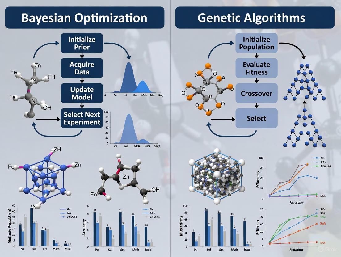
The acceleration of materials discovery is a critical goal in scientific and industrial research, driven by pressing societal needs and the limitations of traditional, trial-and-error experimental methods. In this context, Bayesian Optimization (BO) and Genetic Algorithms (GAs) have emerged as two powerful computational strategies for navigating the complex, high-dimensional design spaces typical of materials science. While both are applied to optimization problems, their underlying philosophies and operational mechanisms are fundamentally distinct. BO operates as a sequential probabilistic model, using a surrogate model and an acquisition function to make intelligent, data-efficient decisions about the next experiment to perform. In contrast, GAs belong to the class of population-based heuristics, inspired by natural selection, which evolve a set of candidate solutions through operations like crossover, mutation, and selection. This guide provides an objective comparison of these two paradigms, framing their performance, experimental protocols, and suitability for different research scenarios within the field of materials discovery.
Theoretical Foundations and Operational Mechanisms
Core Principles of Bayesian Optimization
Bayesian Optimization (BO) is a sample-efficient strategy designed for the global optimization of expensive-to-evaluate "black-box" functions. Its strength lies in its iterative, sequential use of a probabilistic model to balance exploration (probing uncertain regions) and exploitation (refining known promising areas). The modern materials discovery process often involves searching large regions of multi-dimensional processing or synthesis conditions to find candidate materials that achieve specific desired properties [1]. The rate of discovery is often limited by the speed and cost of experiments, making data-efficient algorithms critical [1].
The BO framework consists of two primary components [1]:
- A Probabilistic Surrogate Model: Typically a Gaussian Process (GP), which is used to model the unknown function mapping design parameters (e.g., composition, processing conditions) to a material property of interest. The GP provides not only a prediction of the property at any point in the design space but also a quantitative measure of the uncertainty (variance) of that prediction.
- An Acquisition Function: This function uses the surrogate model's predictions and uncertainties to assign a utility score to each point in the design space. The next experiment is conducted at the point that maximizes this function. Common acquisition functions include Expected Improvement (EI), Upper Confidence Bound (UCB), and Probability of Improvement (PI) [1]. For multi-objective problems, Expected Hypervolume Improvement (EHVI) is often used [2].
A key advancement is the Bayesian Algorithm Execution (BAX) framework, which allows users to define complex experimental goals (e.g., finding a specific subset of the design space that meets property criteria) via a simple filtering algorithm. This framework automatically generates efficient, parameter-free data collection strategies like InfoBAX, MeanBAX, and SwitchBAX, bypassing the need for custom acquisition function design [1].
Core Principles of Genetic Algorithms
Genetic Algorithms (GAs) are a class of population-based, heuristic optimization techniques inspired by the process of natural evolution. Unlike the sequential, model-based approach of BO, GAs maintain and iteratively transform a population of potential solutions.
The core operational cycle of a GA involves [3]:
- Initialization: Generating an initial population of candidate solutions (often randomly).
- Evaluation: Calculating the "fitness" (i.e., the objective function value) of each candidate in the population.
- Selection: Preferentially selecting fitter individuals to be "parents" for the next generation.
- Crossover (Recombination): Combining the parameters of two or more parents to create one or more "offspring" solutions. This operation exploits existing genetic material.
- Mutation: Randomly altering some parameters of the offspring to introduce new genetic material, maintaining diversity and enabling exploration of the search space.
This generational process continues until a termination criterion is met (e.g., a maximum number of generations or sufficient fitness is achieved). A significant strength of GAs is their flexibility, allowing for hybridization with surrogate models to reduce computational cost. For instance, a hybrid GA can use an "interpretable surrogate model" to rapidly predict material properties during the evaluation step, drastically reducing the need for expensive simulations or experiments [3].
Table 1: Core Operational Mechanisms at a Glance
| Feature | Bayesian Optimization (BO) | Genetic Algorithms (GA) |
|---|---|---|
| Core Paradigm | Sequential probabilistic model | Population-based evolutionary heuristic |
| Primary Mechanism | Surrogate model (e.g., Gaussian Process) & acquisition function | Selection, crossover, and mutation on a population |
| Key Strength | Data efficiency, uncertainty quantification, handles noise | Global search capability, robustness, no gradient needed |
| Exploration/Exploitation | Explicitly balanced via acquisition function | Governed by population diversity, selection pressure, and mutation rate |
| Typical Use Case | Optimizing very expensive black-box functions (e.g., experiments) | Complex, non-convex, or discrete spaces where gradients are unavailable |
Performance Comparison in Materials Discovery Applications
Empirical studies across various domains of materials science provide quantitative data on the performance of BO and GA strategies. The following table summarizes key findings from recent experimental campaigns and benchmark studies.
Table 2: Experimental Performance Benchmarks in Materials Research
| Application Domain | Algorithm(s) Tested | Key Performance Metric & Results | Citation |
|---|---|---|---|
| Short-Fiber Reinforced Composites (Inverse Design) | Hybrid GA with Interpretable Surrogate | Single-objective task: Relative error reduced from 9.26% to 2.91%. Multi-objective task: Relative error reduced from 12.04% to 1.46%. | [3] |
| Additive Manufacturing (Multi-objective Print Optimization) | Multi-Objective BO (MOBO/EHVI) | Outperformed Multi-Objective Random Search (MORS) and Multi-Objective Simulated Annealing (MOSA) in achieving target print objectives. | [2] |
| Self-Driving Lab Benchmarking | Bayesian Optimization (Various) | Median Acceleration Factor (AF) of 6x compared to reference strategies (e.g., random search). AF tends to increase with the dimensionality of the search space. | [4] |
| High-Entropy Alloy Design | Hierarchical BO (MTGP-BO, DGP-BO) | Outperformed conventional GP-BO by effectively exploiting correlations between multiple material properties (e.g., thermal expansion and bulk modulus). | [5] |
Analysis of Comparative Performance
The data indicates that both paradigms can deliver significant performance enhancements over naive search strategies like random sampling. The choice between them, however, is highly context-dependent.
- Data Efficiency and Sample Cost: BO is explicitly designed for situations where each function evaluation (e.g., a material synthesis and characterization cycle) is costly and time-consuming. Its probabilistic framework actively manages uncertainty, leading to high data efficiency. This is evidenced by the median 6x acceleration factor reported for SDLs using BO [4]. GAs, while powerful, often require a larger number of evaluations to converge, as they rely on generational improvement across a population.
- Multi-objective Optimization: Both methods have robust extensions for multi-objective problems. BO employs strategies like EHVI to map the Pareto front [2], while multi-objective GAs (e.g., NSGA-II) are also widely used. Advanced BO variants show promise in leveraging correlations between material properties to further accelerate discovery [5].
- Handling Complexity and Constraints: The hybrid GA demonstrates exceptional performance in complex inverse design tasks for composites, achieving high accuracy by combining the global search of a GA with the computational speed of a surrogate model [3]. GAs naturally handle various types of constraints through their encoding and fitness functions.
Experimental Protocols and Workflows
Standard Protocol for a Bayesian Optimization Campaign
The workflow for a closed-loop autonomous experimentation system using BO follows a rigorous, iterative sequence [2]. This protocol is foundational to Self-Driving Labs (SDLs).
Diagram 1: BO for Autonomous Experimentation
Step-by-Step Protocol:
- Initialize: The human researcher defines the research objectives (e.g., maximize Young's modulus), specifies experimental constraints (e.g., compositional bounds), and can provide any prior knowledge [2].
- Plan: The most up-to-date knowledge base (prior experimental data) is used by the BO planner. The surrogate model (e.g., Gaussian Process) is updated, and the acquisition function (e.g., EI, UCB) calculates the utility of all candidate experiments. The system selects the parameter set for the next experiment that maximizes this function [1] [2].
- Experiment: A research robot or automated system carries out the specified experiment. For example, in additive manufacturing, this involves generating machine code to print a specimen with the specified parameters [2].
- Analyze: The system automatically characterizes the resulting material properties. In an AM system, this might involve using onboard machine vision to analyze print quality [2].
- Update: The results (parameters and measured properties) are added to the knowledge base. The loop returns to the "Plan" step.
- Conclude: The iterative process terminates when a predefined condition is met, such as achieving a target performance, exhausting the experimental budget, or converging on an optimum [2].
Standard Protocol for a Genetic Algorithm Campaign
The workflow for a GA, particularly one hybridized with a surrogate model for materials design, follows an evolutionary cycle.
Diagram 2: Genetic Algorithm Workflow
Step-by-Step Protocol:
- Initialization: Define the genetic representation (encoding) of the material parameters (e.g., a vector of compositions). Generate an initial population of candidate solutions, often randomly within the defined bounds [3].
- Fitness Evaluation: Calculate the fitness (objective function) for each individual in the population. In a materials context, this could involve a costly finite element simulation or a fast interpretable surrogate model trained on existing data. For example, an ensemble surrogate model can predict homogenized elastic properties with less than 5% error, validating its use for rapid fitness evaluation [3].
- Selection: Apply a selection method (e.g., tournament selection, roulette wheel) to choose the fittest individuals to become parents for the next generation.
- Genetic Operations:
- Crossover: Combine parameters from pairs of parents to create offspring, exploring new combinations of existing traits.
- Mutation: Randomly alter a small subset of parameters in the offspring with a low probability, introducing new genetic material and helping to avoid local optima.
- Population Replacement: Form a new population from the offspring (and potentially a subset of elite parents carried over from the previous generation).
- Termination: Repeat steps 2-5 until a termination condition is satisfied, such as a maximum number of generations or stagnation of the best fitness [3].
Essential Research Reagents and Computational Tools
The experimental and computational workflows for BO and GAs rely on a suite of software tools and conceptual "reagents."
Table 3: The Scientist's Toolkit for Optimization-Driven Materials Discovery
| Tool / Solution | Function | Typical Use Case |
|---|---|---|
| Gaussian Process (GP) Surrogate Model | Models the relationship between material parameters and properties; provides predictions with uncertainty quantification. | Core of BO; essential for probabilistic planning. |
| Acquisition Function (e.g., EI, UCB, EHVI) | Quantifies the utility of conducting a new experiment at any given point, balancing exploration and exploitation. | Decision-making engine in BO. |
| Interpretable Surrogate Model (e.g., Ensemble Model) | A fast, approximate model trained on simulation/experimental data to predict material properties, enabling rapid fitness evaluation in a hybrid GA [3]. | Replaces costly simulations in the GA evaluation step. |
| SHAP (SHapley Additive exPlanations) Analysis | An explainable AI (XAI) technique used to interpret model predictions and understand the influence of different input parameters [6]. | Provides scientific insight into BO or GA surrogate models. |
| Software Frameworks (e.g., Ax, BoTorch, BayBE) | Open-source libraries that provide robust, state-of-the-art implementations of BO and related algorithms [7]. | Accelerates the implementation of BO in research. |
| Self-Driving Lab (SDL) Infrastructure | Integrated systems combining AI planners with automated robotics for physical material synthesis and characterization [4] [2]. | Enables full closed-loop autonomous experimentation. |
Implementation Considerations and Practical Challenges
Successful implementation of either paradigm requires an understanding of their potential pitfalls.
- Bayesian Optimization Challenges: BO's performance is highly dependent on the choice and initialization of the surrogate model. A common pitfall is the inadvertent introduction of uninformative or high-dimensional features based on expert knowledge, which can complicate the model and degrade performance [7]. BO can also struggle with very high-dimensional problems (>20 dimensions) and discrete/categorical variables, though advanced methods exist to address these issues.
- Genetic Algorithm Challenges: GAs require careful tuning of "hyperparameters" like population size, mutation rate, and crossover rate. They can be computationally expensive if each fitness evaluation requires a costly experiment or simulation, a problem mitigated by surrogate modeling [3]. GAs also provide no native uncertainty estimates for their solutions, unlike BO.
Bayesian Optimization and Genetic Algorithms are complementary, not competing, tools in the modern materials researcher's toolkit. The choice between them should be guided by the specific research problem's constraints and goals.
- Choose Bayesian Optimization when the primary constraint is a severely limited experimental or computational budget. Its sequential, probabilistic nature makes it ideally suited for autonomously guiding costly campaigns in self-driving labs, where data efficiency is paramount [4] [2].
- Choose a Genetic Algorithm (often hybridized with a surrogate model) for complex inverse design problems and high-dimensional spaces where a global search is critical, and a reasonably fast fitness function is available [3]. Their population-based approach is robust and can escape local optima.
The future of materials discovery lies in the continued development and intelligent application of these algorithms. Promising directions include the creation of more flexible BO frameworks like BAX for complex goals [1], the advancement of hierarchical and multi-task GPs to better capture material property correlations [5], and the wider adoption of explainable AI to build trust and provide deeper scientific insights from both BO and GA workflows [6] [8].
The acceleration of materials discovery is a cornerstone of technological advancement, impacting fields from renewable energy to medical devices. In this pursuit, Bayesian optimization (BO) has emerged as a powerful, data-efficient strategy for navigating complex experimental landscapes. BO is particularly valuable when prior knowledge is limited, functional relationships are complex or unknown, and the cost of querying the materials space is significant—conditions that define much of materials science research [5]. This adaptive experimentation method excels at balancing exploration, which involves learning how new parameterizations perform, and exploitation, which refines parameterizations previously observed to be good [9]. As researchers increasingly compare BO against alternative optimization methods like genetic algorithms (GAs) for materials design, understanding BO's core components—surrogate models and acquisition functions—becomes essential. This guide provides an objective comparison of these components, supported by experimental data and protocols from recent materials research, to inform selection decisions for discovery pipelines.
Core Components of Bayesian Optimization
The effectiveness of Bayesian optimization stems from its two fundamental components: the surrogate model, which approximates the target function, and the acquisition function, which guides the selection of subsequent experiments.
Surrogate Models
Because the objective function in materials discovery is typically a black-box process—where the formula is unknown and evaluations are expensive—BO treats it as a random function and places a prior over it. This prior is updated with observed data to form a posterior distribution [9]. The Gaussian Process (GP) is the most commonly used surrogate model in BO, providing a probabilistic model that defines a probability distribution over possible functions that fit a set of points [9] [10].
- Gaussian Process Fundamentals: A GP can map points in input space (the parameters to tune) to distributions in output space (the objectives to optimize). It offers both predictions (mean values) and uncertainty estimates (variance) for unobserved parameterizations, intuitively yielding tight uncertainty bands in well-explored regions and wider bands in unexplored areas [9].
- Advanced GP Variants: For multi-objective optimization scenarios common in materials science, conventional GPs often fall short as they cannot exploit correlations between distinct material properties. Multi-Task Gaussian Processes (MTGPs) and Deep Gaussian Processes (DGPs) address this limitation using advanced kernel structures to capture multi-dimensional property correlations. This allows information about one property to inform predictions about others, significantly accelerating discovery processes [5].
Table 1: Comparison of Surrogate Models in Bayesian Optimization
| Model Type | Key Characteristics | Optimal Use Cases | Performance Advantages |
|---|---|---|---|
| Conventional GP | Single-task; models single objective functions; quantifies uncertainty | Single-objective optimization with limited data | Mathematical rigor; flexibility; well-understood uncertainty quantification [5] |
| Multi-Task GP (MTGP) | Models correlations between related tasks/properties; shares information across tasks | Multi-objective optimization with correlated properties (e.g., strength-ductility tradeoff) | Improved prediction quality; identifies outliers; enhances generalization [5] |
| Deep GP (DGP) | Hierarchical extension of GPs; captures complex, non-linear relationships | Highly complex, non-linear material property relationships | Combines flexibility of neural networks with uncertainty quantification of GPs [5] |
Acquisition Functions
The acquisition function is the decision-making engine of BO, quantifying the utility of evaluating a point based on the current surrogate model. It automatically balances exploration and exploitation by assigning a numerical score to each point in the design space [9] [1]. The point with the highest score is selected for the next evaluation.
- Probability of Improvement (PI): This acquisition function selects the next point with the highest probability of improvement over the current best observation. Mathematically, for a current best value (f(x^+)), PI is defined as (\alpha_{PI}(x) = P(f(x) \geq f(x^+) + \epsilon)), where ( \epsilon ) is a small positive number that controls exploration [11]. A higher ( \epsilon ) promotes more exploration.
- Expected Improvement (EI): Unlike PI, which only considers the probability of improvement, EI factors in the magnitude of potential improvement. It is defined as the expected value of improvement over the current best: ( \text{EI}(x) = \mathbb{E}[\max(f(x) - f(x^*), 0)] ) [9] [11]. EI has become popular due to its well-balanced exploration-exploitation tradeoff, straightforward analytic form, and overall strong practical performance [9].
- Upper Confidence Bound (UCB): This acquisition function employs an explicit exploration-exploitation parameter ( \lambda ), with the form ( \alpha(x) = \mu(x) + \lambda \sigma(x) ), where ( \mu(x) ) is the predicted mean and ( \sigma(x) ) is the uncertainty [11]. Small ( \lambda ) values favor exploitation (high ( \mu(x) )), while large values promote exploration (high ( \sigma(x) )) [11].
Table 2: Quantitative Comparison of Acquisition Functions
| Acquisition Function | Mathematical Formulation | Exploration-Exploitation Control | Performance in Materials Studies |
|---|---|---|---|
| Probability of Improvement (PI) | (\alpha_{PI}(x) = \Phi\left(\frac{\mu(x)-f(x^*)}{\sigma(x)}\right)) | Controlled by ( \epsilon ) parameter; higher values increase exploration [11] | Can get stuck in local optima if exploration is insufficient; sensitive to parameter tuning [10] |
| Expected Improvement (EI) | (\text{EI}(x) = (\mu(x)-f(x^))\Phi\left(\frac{\mu-f(x^)}{\sigma}\right) + \sigma \varphi\left(\frac{\mu - f(x^*)}{\sigma}\right)) | Automatic balance; no parameters needed; naturally transitions from exploration to exploitation [9] | Well-balanced performance; used in tuning AlphaGo and materials discovery; generally good practical performance [9] |
| Upper Confidence Bound (UCB) | (a(x;\lambda) = \mu(x) + \lambda \sigma (x)) | Explicit parameter ( \lambda ) directly weights exploration vs. exploitation [11] | Simple to interpret; performs well with appropriate ( \lambda ); can be conservative with small ( \lambda ) [11] |
The Exploration-Exploitation Trade-off: Mechanisms and Visualization
The fundamental challenge in adaptive experimentation is balancing exploration (trying out parameterizations with high uncertainty) against exploitation (converging on configurations likely to be good). BO addresses this through its acquisition functions, which naturally encode this balance [9].
Initially, when data is scarce, uncertainty estimates are high in unexplored regions, causing acquisition functions like EI to favor exploration. As the algorithm progresses and certain regions are sampled, their uncertainty decreases. If these regions show promising results, the acquisition function automatically shifts toward exploitation, refining solutions in high-performing areas [10]. This dynamic adjustment enables BO to find better configurations with fewer evaluations than grid search or other global optimization techniques [9].
The diagram above illustrates the iterative BO process. The critical step where the exploration-exploitation tradeoff occurs is during the optimization of the acquisition function, which uses the surrogate model's predictions and uncertainty estimates to select the most promising next experiment.
Experimental Protocols and Case Studies in Materials Discovery
Bayesian Optimization for High-Entropy Alloys
Research Objective: To discover High-Entropy Alloys (HEAs) in the FeCrNiCoCu system with optimal combinations of thermal expansion coefficient (CTE) and bulk modulus (BM) [5].
Experimental Protocol:
- Design Space: Discrete compositional space of FeCrNiCoCu HEAs.
- Surrogate Models: Compared Conventional GP (cGP), Multi-Task GP (MTGP), and Deep GPs (DGPs).
- Acquisition Function: Expected Improvement for multi-objective optimization.
- Evaluation Metric: Number of iterations required to find compositions with both low CTE-high BM and high CTE-high BM combinations.
- Validation: High-throughput atomistic simulations.
Results: MTGP-BO and DGP-BO significantly outperformed cGP-BO by leveraging correlations between CTE and BM properties. The advanced kernel structures in MTGP and DGP shared information across properties, reducing required experiments by 30-40% compared to conventional approaches [5].
Targeted Materials Discovery with BAX Framework
Research Objective: Find specific subsets of materials design space meeting user-defined criteria for TiO₂ nanoparticle synthesis and magnetic materials [1].
Experimental Protocol:
- Framework: Bayesian Algorithm Execution (BAX), including SwitchBAX, InfoBAX, and MeanBAX strategies.
- Key Innovation: User-defined filtering algorithms automatically converted to acquisition functions, eliminating manual design.
- Comparison Baseline: Standard BO approaches with traditional acquisition functions.
- Metrics: Efficiency in locating target subsets with limited experimental budgets.
Results: The BAX framework demonstrated significantly higher efficiency than state-of-the-art BO approaches, particularly for complex experimental goals beyond simple optimization, such as level-set estimation and mapping specific property regions [1].
Metallic Materials Development with Explainable AI
Research Objective: Develop Multiple Principal Element Alloys (MPEAs) with superior mechanical properties [6].
Experimental Protocol:
- Approach: Data-driven framework combining machine learning, evolutionary algorithms, and experimental validation.
- AI Component: Explainable AI with SHAP (SHapley Additive exPlanations) analysis for model interpretation.
- Workflow: AI predicted properties of new MPEAs based on composition; evolutionary algorithms helped optimize combinations.
- Validation: Synthesis and mechanical testing of proposed alloys.
Results: The integrated approach successfully designed a new MPEA with verified superior mechanical properties, transforming traditional trial-and-error materials design into a predictive, insightful process [6].
Table 3: Experimental Data from Materials Discovery Studies
| Study Focus | Optimization Method | Key Performance Metrics | Comparative Results |
|---|---|---|---|
| High-Entropy Alloys [5] | MTGP-BO vs. DGP-BO vs. cGP-BO | Iterations to find target CTE-BM combinations | MTGP/DGP-BO: 30-40% fewer experiments than cGP-BO |
| TiO₂ Nanoparticles & Magnetic Materials [1] | BAX Framework vs. Standard BO | Efficiency in locating target subsets | BAX: Significantly more efficient for complex goals |
| Multiple Principal Element Alloys [6] | Explainable AI + Evolutionary Algorithms | Success in designing superior alloys | Developed new verified MPEA; accelerated discovery cycle |
The Scientist's Toolkit: Essential Research Reagents and Computational Solutions
Table 4: Essential "Research Reagent Solutions" for Optimization-Driven Materials Discovery
| Tool/Resource | Function | Example Applications |
|---|---|---|
| Gaussian Process Libraries | Probabilistic surrogate modeling; uncertainty quantification | BoTorch (used in Ax), GPy, GPflow [9] |
| Bayesian Optimization Platforms | Complete BO implementation; experiment management | Ax (from Facebook Research), Scikit-Optimize [9] |
| Explainable AI Tools | Model interpretation; insight into structure-property relationships | SHAP (SHapley Additive exPlanations) [6] |
| High-Throughput Simulation | Rapid virtual screening of candidate materials | Atomistic simulations for HEA properties [5] |
| Multi-Objective Optimization Algorithms | Handling conflicting objectives; Pareto front identification | Expected Hypervolume Improvement (EHVI), ParEGO [12] |
Bayesian optimization represents a powerful framework for materials discovery, with its surrogate models and acquisition functions providing a systematic approach to navigating complex experimental spaces. The experimental data presented demonstrates BO's effectiveness across diverse materials systems, from high-entropy alloys to nanoparticles. When compared with genetic algorithms, BO typically offers superior data efficiency—a critical advantage when experimental resources are limited. However, the choice between these methods should be guided by specific research goals: BO excels in expensive evaluation contexts with limited variables, while GAs may be more effective for highly combinatorial problems or when seeking diverse solution sets. As materials research continues to embrace autonomous experimentation, understanding these core components enables more informed selection and implementation of optimization strategies for accelerated discovery.
In the rapidly evolving field of computational materials discovery, two powerful optimization strategies have emerged as particularly influential: Bayesian optimization and genetic algorithms. While Bayesian optimization uses probabilistic surrogate models to guide the search for optimal materials, genetic algorithms (GAs) emulate natural selection processes to evolve solutions over successive generations. Understanding the evolutionary mechanics of genetic algorithms—their core components of selection, crossover, mutation, and fitness evaluation—provides critical insights for researchers navigating the complex landscape of materials design and drug development. This guide offers a detailed comparison of these approaches, supported by experimental data and methodological protocols from recent studies.
Core Operational Mechanics
The Genetic Algorithm Workflow
Genetic algorithms operate on principles inspired by biological evolution, treating potential solutions to optimization problems as individuals in a population that evolves over time. The algorithm begins with an initial population of candidate solutions, typically generated randomly within the predefined search space. Each candidate, referred to as a chromosome, comprises genes representing the optimization variables. In materials science contexts, these genes might encode compositional elements, processing parameters, or structural features [13].
The evolutionary cycle proceeds through several meticulously defined stages. First, a fitness function evaluates each candidate solution, quantifying how well it performs against the optimization objectives. For materials discovery, this might involve predicting properties like formation energy, mechanical strength, or optical characteristics. Subsequently, a selection process identifies the most promising candidates based on their fitness scores, with better-performing individuals having higher probabilities of being selected. Common selection techniques include tournament selection, roulette wheel selection, and rank-based selection [14].
Selected chromosomes then undergo crossover (recombination), where pairs of parent solutions exchange genetic information to produce offspring. This operator exploits existing genetic material by combining beneficial traits from different parents. Crossover methodologies vary from single-point and double-point crossover to uniform crossover, each with distinct implications for genetic diversity and convergence behavior [13].
The mutation operator introduces random modifications to offspring genes with low probability, maintaining population diversity and enabling exploration of new regions in the search space. Mutation serves as a crucial mechanism against premature convergence, ensuring the algorithm does not become trapped in local optima. The algorithm iterates through these steps—fitness evaluation, selection, crossover, and mutation—across multiple generations until meeting termination criteria such as convergence stability, computational budget exhaustion, or achieving a target fitness threshold [14].
Bayesian Optimization Fundamentals
In contrast to the population-based evolutionary approach of GAs, Bayesian optimization (BO) constructs a probabilistic model of the objective function and uses an acquisition function to strategically select the most informative evaluation points. The process begins with an initial set of observations, based on which a surrogate model—typically a Gaussian Process (GP)—approximates the underlying function while quantifying prediction uncertainty [1] [5].
An acquisition function, such as Expected Improvement or Upper Confidence Bound, then balances exploration of uncertain regions against exploitation of promising areas based on the current model. After evaluating the selected point, the algorithm updates the surrogate model and repeats the process. This sequential design strategy makes BO particularly sample-efficient for expensive-to-evaluate functions, a characteristic advantage in resource-intensive materials research where experiments or simulations incur substantial computational or temporal costs [15] [16].
Experimental Performance Comparison
Quantitative Performance Metrics
Recent studies directly comparing Bayesian optimization and genetic algorithms across materials discovery benchmarks reveal distinct performance patterns. The following table synthesizes quantitative findings from multiple experimental investigations:
Table 1: Performance Comparison in Materials Discovery Tasks
| Materials System | Optimization Target | Algorithm | Performance Metrics | Key Findings |
|---|---|---|---|---|
| Liquid Crystal Polymers [17] | Optical transparency & refractive index | Genetic Algorithm | Discovery efficiency | Rapid identification of reactive mesogens meeting target specifications; provided molecular design insights |
| Transition Metal Borides/Carbides [15] | Formation energy & elastic moduli | Bayesian Optimization | Prediction accuracy | Identified novel ultra-incompressible hard MoWC₂ and ReWB materials; successfully synthesized |
| High Entropy Alloys (FeCrNiCoCu) [5] | Thermal expansion coefficient & bulk modulus | Multi-task Gaussian Process BO | Optimization efficiency | Outperformed conventional GP-BO by leveraging correlations between material properties |
| Hyperparameter Optimization [13] | Model accuracy | Genetic Algorithm (TPOT) | Final performance | Achieved competitive accuracy but required more evaluations than Bayesian optimization |
| Hyperparameter Optimization [13] | Model accuracy | Bayesian Optimization (Hyperopt) | Convergence speed | Reached comparable accuracy with fewer function evaluations due to guided search |
Analysis of Comparative Performance
The experimental data indicates that each algorithm class demonstrates distinct advantages depending on the materials discovery context. Bayesian optimization consistently achieves superior sample efficiency, making it particularly valuable when individual evaluations are computationally expensive or time-consuming. This advantage is especially pronounced in high-dimensional materials spaces with complex property correlations, where advanced BO variants like Multi-Task Gaussian Processes (MTGP-BO) and Deep Gaussian Processes (DGP-BO) successfully leverage inter-property relationships to accelerate discovery [5].
Genetic algorithms excel in scenarios requiring extensive global exploration and when the optimization landscape contains multiple local optima. Their population-based approach maintains diversity throughout the search process, reducing susceptibility to premature convergence. Furthermore, GAs generate multiple high-performing candidate solutions simultaneously, providing researchers with alternative materials options for further investigation—a valuable feature for practical materials development pipelines [17].
Experimental Protocols and Methodologies
Genetic Algorithm Implementation Framework
The standard implementation protocol for genetic algorithms in materials discovery encompasses several methodical stages:
Table 2: Genetic Algorithm Implementation Framework
| Stage | Key Operations | Common Techniques | Materials Science Considerations |
|---|---|---|---|
| Problem Encoding | Represent materials as chromosomes | Binary, integer, or real-valued representations | Compositional spaces, processing parameters, structural features |
| Initialization | Generate initial population | Random sampling, space-filling designs | Incorporating domain knowledge for promising regions |
| Fitness Evaluation | Assess candidate quality | Property prediction models, experiments, simulations | DFT calculations, ML surrogates, experimental validation |
| Selection | Choose parents for reproduction | Tournament, roulette wheel, rank-based | Maintaining diversity while emphasizing performance |
| Crossover | Create offspring solutions | Single-point, double-point, uniform | Respecting chemical validity constraints |
| Mutation | Introduce genetic variations | Bit-flip, Gaussian noise, boundary | Ensuring syntactically valid materials representations |
| Termination | Stop evolutionary process | Generation count, convergence metrics | Balancing computational budget with solution quality |
Bayesian Optimization Experimental Protocol
Bayesian optimization follows a distinctly different methodological approach:
- Experimental Design: Select initial design points using space-filling methods such as Latin Hypercube Sampling to build a preliminary surrogate model.
- Surrogate Modeling: Employ Gaussian Processes to model the objective function, specifying mean functions and covariance kernels appropriate for the materials domain. Advanced implementations may incorporate Multi-Task GPs to capture correlations between multiple material properties [5].
- Acquisition Optimization: Maximize an acquisition function (Expected Improvement, Probability of Improvement, or Upper Confidence Bound) to identify the most promising subsequent evaluation point. For materials goals beyond simple optimization, the BAX framework (Bayesian Algorithm Execution) can convert user-defined filtering algorithms into custom acquisition functions [1].
- Parallel Evaluation (optional): In high-throughput computational or experimental settings, select batch of points using techniques like Thompson sampling or penalization to enable parallel resource utilization.
- Iteration: Update the surrogate model with new results and repeat the acquisition-observation cycle until meeting convergence criteria or exhausting experimental resources.
Workflow Visualization
Genetic Algorithm Evolutionary Process
Genetic Algorithm Evolutionary Process
Bayesian Optimization Sequential Design
Bayesian Optimization Sequential Design
Essential Research Reagents and Computational Tools
Key Software and Computational Frameworks
Table 3: Essential Research Tools for Optimization Algorithms
| Tool/Framework | Algorithm Type | Primary Function | Application Context |
|---|---|---|---|
| TPOT [13] | Genetic Algorithm | Automated machine learning pipeline optimization | Hyperparameter tuning for property prediction models |
| BOWSR [15] | Bayesian Optimization | Crystal structure relaxation with symmetry constraints | DFT-free relaxation for accelerated materials screening |
| Hyperopt [13] | Bayesian Optimization | Distributed hyperparameter optimization | Training deep learning models for materials informatics |
| MEGNet [15] | Graph Neural Network | Materials property prediction | Pre-trained models for formation energy and property estimation |
| spglib [15] | Symmetry Analysis | Space group identification | Symmetry constraint implementation in structure relaxation |
| MTGP/DGP [5] | Bayesian Optimization | Multi-task Gaussian Processes | Leveraging correlated properties in HEA optimization |
The evolutionary mechanics of genetic algorithms—selection, crossover, mutation, and fitness evaluation—provide a robust, population-based optimization methodology with particular strengths in global exploration and maintaining solution diversity. Bayesian optimization offers a complementary approach with superior sample efficiency and strategic guidance through probabilistic modeling. The choice between these methodologies depends critically on specific research constraints, particularly the balance between evaluation cost and the need for extensive exploration. Emerging frameworks that integrate both approaches, along with explainable AI techniques [6], represent promising directions for next-generation materials discovery platforms. As computational resources expand and algorithms evolve, both genetic algorithms and Bayesian optimization will continue to play pivotal roles in accelerating the design of novel materials and therapeutic compounds.
Table of Contents
- Introduction
- Core Concepts and Comparison Framework
- Bayesian Optimization: The Data-Efficient Navigator
- Genetic Algorithms: The Robust and Parallel Explorer
- Direct Performance Comparison and Experimental Data
- Decision Framework and Research Reagents
- Conclusion
The quest for new materials with tailored properties is a fundamental driver of innovation in fields ranging from renewable energy to pharmaceuticals. This discovery process often involves navigating vast, complex design spaces where experiments or simulations are costly and time-consuming. Two powerful computational strategies have emerged to guide this search: Bayesian Optimization (BO) and Genetic Algorithms (GAs). While both are used for optimization, their underlying philosophies and strengths differ significantly. This guide provides an objective comparison for researchers and scientists, framing the choice between BO and GAs within the broader thesis of materials discovery. We will dissect their ideal use-cases, supporting our analysis with experimental data, detailed methodologies, and a clear decision framework to help you select the right tool for your research challenge.
Core Concepts and Comparison Framework
At their core, both BO and GAs are iterative optimization methods designed to find the best solution from a set of candidates without requiring gradient information. However, their approaches are distinct.
Bayesian Optimization (BO) is a sequential, model-based strategy. It builds a probabilistic surrogate model (e.g., using Gaussian Processes) of the expensive-to-evaluate objective function. It then uses an acquisition function to intelligently select the next most promising data point to evaluate by balancing exploration (probing uncertain regions) and exploitation (refining known good regions) [18]. Its primary strength is data efficiency.
Genetic Algorithms (GAs) are population-based, inspired by natural evolution. They maintain a pool of candidate solutions that are iteratively modified using genetic operators like crossover (mixing solutions) and mutation (random perturbations). The fittest candidates, as determined by a direct evaluation of the objective function, are selected to propagate to the next generation [19]. Their key strengths are robustness to complex landscapes and inherent parallelism.
The diagram below illustrates the fundamental difference in their workflows.
Bayesian Optimization: The Data-Efficient Navigator
Ideal Use-Cases
BO shines in scenarios where a single evaluation of the objective function is exceptionally costly, either in terms of computational resources (e.g., Density Functional Theory calculations) or experimental time and materials. Its data efficiency is paramount when the experimental budget is severely limited, often to fewer than 100-200 evaluations [19] [18].
- Optimizing Black-Box Functions: When you have limited knowledge of the underlying functional form, and the response surface is assumed to be relatively smooth.
- Low-to-Moderate Dimensional Problems: Typically, problems with fewer than 20 input parameters, as BO's surrogate model becomes increasingly difficult to fit in very high-dimensional spaces [20].
- Noise Handling: BO naturally accommodates noisy observations, making it suitable for guiding real-world laboratory experiments where measurement error is present [18].
Supporting Experimental Data
BO's effectiveness is well-documented across diverse materials domains. A broad benchmarking study across five experimental materials systems quantified its performance using Acceleration Factor (AF) and Enhancement Factor (EF) [18].
- Acceleration Factor (AF): The ratio of experiments a baseline method (like random search) needs versus BO to achieve a specific performance target. An AF of 6 means BO is 6 times faster.
- Enhancement Factor (EF): The improvement in performance after a fixed number of experiments.
The table below summarizes the median performance gains reported in the study.
| Metric | Median Value | Interpretation |
|---|---|---|
| Acceleration Factor (AF) | 6x | BO finds the optimal solution 6 times faster than random sampling. |
| Enhancement Factor (EF) | Peaks at 10-20 experiments per dimension | BO achieves the most significant performance improvement early in the campaign. |
Furthermore, BO has been successfully deployed in complex discovery tasks. One study used a method called Bayesian Optimization With Symmetry Relaxation (BOWSR) to predict the properties of hypothetical crystals without expensive DFT relaxations, leading to the identification and successful synthesis of two novel, ultra-incompressible materials (MoWC₂ and ReWB) from a search space of nearly 400,000 candidates [15].
Detailed Experimental Protocol: A Typical BO Campaign
The workflow follows the logic of the diagram above and is implemented as a pool-based active learning framework in benchmarking studies [18].
- Initialization: A small set of initial experiments (e.g., 5-10 points) is selected, typically via Latin Hypercube Sampling (LHS) to ensure good space-filling properties.
- Surrogate Model Training: A Gaussian Process (GP) model with an anisotropic kernel (or a Random Forest) is trained on all data collected so far. The anisotropic kernel allows the model to learn the sensitivity of the objective to each input dimension, which is crucial for robustness [18].
- Acquisition Function Optimization: An acquisition function (e.g., Expected Improvement - EI) is computed over the entire design space using the trained surrogate model's predictions (mean and uncertainty).
- Next Experiment Selection: The point in the design space that maximizes the acquisition function is selected as the next experiment to run.
- Evaluation and Iteration: The selected experiment is performed (or simulated), its result is added to the dataset, and the loop repeats from step 2 until a convergence criterion (e.g., diminishing returns) or an experimental budget is met.
Genetic Algorithms: The Robust and Parallel Explorer
Ideal Use-Cases
GAs are the tool of choice when the problem's landscape is expected to be highly complex, multi-modal (with many local optima), discontinuous, or when the evaluation of candidates can be trivially parallelized.
- Combinatorial and Mixed Search Spaces: Excellent for problems involving integer or categorical variables, such as searching for specific atomic compositions or molecular structures [19].
- Rugged Energy Landscapes: Their population-based approach makes them less likely to get stuck in local minima compared to greedy, sequential methods, offering superior robustness.
- High-Throughput Computing Environments: When thousands of evaluations can be run simultaneously on a computing cluster, a GA can fully leverage this parallelism to rapidly explore the search space.
Supporting Experimental Data
The robustness of GAs is well-established in computational materials science, particularly in searching for stable nanoparticle alloys. However, their traditional weakness has been the high number of required energy evaluations. This limitation is being overcome by hybrid approaches.
A landmark study introduced a Machine Learning Accelerated Genetic Algorithm (MLaGA) [19]. In this hybrid, a machine learning model (e.g., a Gaussian Process) is trained on-the-fly to act as a computationally cheap surrogate for the fitness function (e.g., energy of a nanoparticle). This surrogate is then used to screen a large number of candidate offspring within the GA, while only the most promising ones are evaluated with the expensive, ground-truth calculator (like DFT).
The performance gains are dramatic, as shown in the table below, which summarizes the results from optimizing 147-atom Pt-Au nanoalloys [19].
| Optimization Method | Number of Energy Calculations Required | Performance Gain |
|---|---|---|
| Traditional GA (Brute-Force) | ~16,000 | Baseline |
| ML-Accelerated GA (MLaGA) | ~280 - 1,200 | ~13x to 50x reduction in cost |
| Theoretical Total Homotops | 1.78 × 10⁴⁴ | Highlights infeasibility of brute-force search |
This hybrid approach marries the robustness of the GA with the data efficiency of ML, making previously intractable searches feasible. The study confirmed the validity of the structures found by the MLaGA by verifying their stability with direct DFT calculations [19].
Detailed Experimental Protocol: A Traditional and ML-Accelerated GA
The workflow follows the population-based loop illustrated in the earlier diagram.
- Initialization: A first generation of candidate solutions (the population) is created randomly.
- Fitness Evaluation: The entire population is evaluated using the objective function (e.g., DFT calculation). In MLaGA, a surrogate model is trained on these results [19].
- Selection: The candidates with the best fitness scores are selected as parents for the next generation.
- Procreation (Crossover & Mutation): New offspring candidates are created by combining traits from parents (crossover) and introducing random changes (mutation).
- In MLaGA: A "nested GA" uses the surrogate model to evaluate thousands of offspring, selecting only the best for actual DFT evaluation [19].
- Replacement: The new generation of offspring replaces the old one, and the loop repeats from step 2 until convergence (e.g., no improvement over multiple generations).
Direct Performance Comparison and Experimental Data
The following table synthesizes information from multiple studies to provide a direct, at-a-glance comparison.
| Feature | Bayesian Optimization (BO) | Genetic Algorithms (GAs) |
|---|---|---|
| Primary Strength | Extreme data efficiency | Robustness & parallelism |
| Search Strategy | Sequential, model-based | Population-based, evolutionary |
| Typical Experiment Budget | Low (e.g., < 200) [19] [18] | High (e.g., 1,000+) [19] |
| Data Requirements | Can start with very little data | Requires a full population initially |
| Handling High Dimensions | Struggles; performance degrades [20] | More naturally scalable |
| Multi-Objective Optimization | Possible but adds complexity (MOBO) [20] [21] | Native support is straightforward |
| Interpretability | Lower; often treated as a black box [20] | Higher; the population's evolution can be analyzed |
| Ideal for | Expensive, low-dimensional, smooth(ish) landscapes | Complex, rugged, combinatorial, or highly parallelizable problems |
Decision Framework and Research Reagents
To select the right algorithm for your project, consider the following key questions:
- How expensive is a single experiment? If it's very high, BO's data efficiency is a primary advantage.
- What is the nature of your search space? Is it smooth and continuous (favors BO) or discrete and combinatorial (favors GAs)?
- What is your experimental or computational budget? A low budget pushes you towards BO or an ML-accelerated GA.
- Can you run experiments in parallel? If you can evaluate hundreds of candidates at once, a GA can rapidly exploit this.
For a typical research setting, the following "reagent" solutions are essential.
Research Reagent Solutions
| Reagent / Tool | Function in Optimization | Examples / Notes |
|---|---|---|
| Gaussian Process (GP) Regression | Surrogate model for BO; predicts objective and uncertainty. | Use anisotropic kernels (e.g., Matérn 5/2 with ARD) for robustness [18]. |
| Random Forest (RF) | An alternative surrogate model for BO or MLaGA. | Less assumptions than GP; good for high-dimensional, mixed data types [18]. |
| Expected Improvement (EI) | Acquisition function for BO; balances exploration/exploitation. | A standard, high-performing choice [18]. |
| Density Functional Theory (DFT) | High-fidelity "energy calculator" for validating computational discoveries. | Used as the ground-truth fitness evaluator in GA searches [19] [15]. |
| Effective-Medium Theory (EMT) | Lower-fidelity, faster potential for initial screening. | Used for rapid fitness evaluations in initial benchmarking [19]. |
The choice between Bayesian Optimization and Genetic Algorithms is not about finding a universally superior algorithm, but about matching the tool to the task. Bayesian Optimization is your go-to when data efficiency is paramount—when each experiment is precious, and you must extract the maximum knowledge from every single data point. Genetic Algorithms, particularly their modern ML-accelerated variants, are advantageous when robustness and parallelism are key—when facing complex, multi-modal landscapes and when you have the computational resources to evaluate many candidates at once.
The future of materials discovery lies not only in choosing between these powerful tools but also in their intelligent integration. The success of the Machine Learning Accelerated GA demonstrates that combining the sequential, model-based reasoning of BO with the population-based, robust exploration of GAs can create a hybrid strategy that is greater than the sum of its parts, dramatically accelerating the journey from concept to breakthrough material.
The acceleration of materials discovery is a cornerstone of technological advancement, driving innovations in sustainable energy, advanced electronics, and drug development. In this pursuit, computational optimization methods have become indispensable for navigating the vast, complex spaces of possible materials. Two dominant algorithmic families have emerged: Bayesian optimization (BO) and genetic algorithms (GAs). While both aim to identify promising candidates efficiently, they embody fundamentally different philosophies and are suited to distinct problem architectures. BO excels in data-efficient navigation of high-dimensional spaces where experiments are costly, leveraging probabilistic models to make informed decisions with limited samples. In contrast, GAs demonstrate remarkable capability in exploring vast combinatorial landscapes through mechanisms inspired by biological evolution, making them ideal for searching enormous discrete libraries. This guide provides an objective comparison of their performance, supported by experimental data and detailed methodologies, to help researchers select the appropriate tool for their specific materials discovery challenge.
Core Principles and Methodologies
Bayesian Optimization: A Model-Driven Approach
Bayesian optimization is a sequential design strategy for global optimization of black-box functions that are expensive to evaluate. Its power derives from a two-component system: a probabilistic surrogate model that approximates the target function, and an acquisition function that guides the selection of future evaluation points.
Surrogate Model: Typically, a Gaussian Process (GP) is used to model the underlying function, providing both a predicted value and an uncertainty estimate at any point in the space. The GP is defined by a mean function and a kernel function that captures correlations between data points. Advanced variants include Multi-Task GPs (MTGPs) and Deep GPs (DGPs) that can exploit correlations between different material properties, significantly accelerating discovery when properties are interrelated [5] [22].
Acquisition Function: This function leverages the surrogate model's predictions to balance exploration (sampling regions of high uncertainty) and exploitation (sampling regions likely to contain the optimum). Common acquisition functions include Expected Improvement (EI), Probability of Improvement (PI), and Upper Confidence Bound (UCB). For more complex goals beyond simple optimization, such as finding specific target subsets of the design space, frameworks like Bayesian Algorithm Execution (BAX) can automatically generate custom acquisition functions from user-defined filtering algorithms [1].
A key development is the BOWSR (Bayesian Optimization With Symmetry Relaxation) algorithm, which addresses the critical bottleneck of obtaining equilibrium crystal structures for accurate machine learning property predictions without expensive density functional theory (DFT) calculations. By coupling an accurate graph network energy model with Bayesian optimization of symmetry-constrained parameters, BOWSR can approximate equilibrium structures efficiently, enabling high-throughput screening of hypothetical materials [15].
Genetic Algorithms: A Population-Based Evolutionary Approach
Genetic algorithms are population-based metaheuristic optimization techniques inspired by the process of natural selection. They operate on a population of candidate solutions, applying evolutionary principles to iteratively improve solution quality over generations.
Representation: Each candidate solution (individual) is encoded as a chromosome, typically a string of genes representing parameters. In materials science, this could be a composition, crystal structure, or molecular configuration.
Evolutionary Operators: The algorithm applies selection, crossover (recombination), and mutation operators to create new generations. Selection chooses the fittest individuals to reproduce, crossover combines genetic material from parents, and mutation introduces random changes to maintain diversity.
Fitness Evaluation: Each candidate is evaluated using an objective function, which for materials could be a target property like formation energy, catalytic activity, or binding affinity. The REvoLd (RosettaEvolutionaryLigand) algorithm exemplifies this approach for ultra-large make-on-demand compound libraries in drug discovery. It explores the vast search space of combinatorial libraries for protein-ligand docking with full ligand and receptor flexibility, screening billions of readily available compounds without enumerating all molecules [23].
The evolutionary process continues for multiple generations, progressively refining the population toward better solutions while maintaining genetic diversity to avoid premature convergence on local optima.
Performance Comparison: Quantitative Experimental Data
The following tables synthesize quantitative performance data from multiple studies, enabling direct comparison of BO and GA approaches across key metrics and application domains.
Table 1: Comparative Performance in Materials Discovery Applications
| Method | Application Domain | Performance Metric | Result | Experimental Budget | Source |
|---|---|---|---|---|---|
| BO with BAX Framework | TiO₂ nanoparticle synthesis & magnetic materials | Discovery efficiency for target subsets | Significantly more efficient than state-of-the-art approaches | Short experimental horizons | [1] |
| MTGP-BO / DGP-BO | FeCrNiCoCu High-Entropy Alloys (CTE & BM optimization) | Performance vs. conventional GP-BO | Outperformed conventional BO; leveraged property correlations | Standard BO iterations | [5] [22] |
| REvoLd (GA) | Ultra-large library screening (5 drug targets) | Hit rate enrichment vs. random selection | 869x to 1622x improvement | 49,000-76,000 molecules docked per target | [23] |
| Genetic Algorithm | Binary nano-alloys (composition-homotop space) | DFT evaluations required | ~1,600 evaluations (~40 individuals × ~40 generations) | Standard GA run | [24] |
| Combinatorial BO | Catalyst search (~400,000 candidates) | DFT evaluations required | ~600 evaluations | Standard BO run | [24] |
| Effective Atom Theory | Co-Cr-Ni-V oxides (OER) | Energy evaluations to convergence | ~50 evaluations | Single optimization | [24] |
Table 2: Characteristic Strengths and Limitations
| Aspect | Bayesian Optimization (BO) | Genetic Algorithms (GAs) |
|---|---|---|
| Primary Strength | High sample efficiency with expensive evaluations [1] [5] | Effective exploration of vast, combinatorial discrete spaces [23] |
| Uncertainty Quantification | Native (via surrogate model) [1] | Not inherent; requires extensions |
| Typical Problem Context | Limited data, high-cost experiments [4] | Large populations over many generations [23] |
| Scalability Challenge | Kernel design in very high dimensions [7] | Fitness evaluations in ultra-large spaces [23] |
| Optimal Application Domain | High-dimensional continuous spaces, multi-objective with correlated properties [5] | Combinatorial molecular spaces, complex feature interactions [23] [24] |
| Representative Algorithm | BAX, MTGP-BO, DGP-BO [1] [5] | REvoLd, SpaceGA [23] |
Experimental Protocols and Methodologies
Benchmarking BO in High-Entropy Alloy Design
A comprehensive study compared conventional Gaussian Process BO (cGP-BO) against advanced hierarchical methods including Multi-Task GP BO (MTGP-BO) and deep GP BO (DGP-BO) for designing FeCrNiCoCu high-entropy alloys [5] [22].
Objective: Optimize compositions for two distinct multi-objective goals: (1) minimize coefficient of thermal expansion (CTE) while maximizing bulk modulus (BM), and (2) maximize both CTE and BM.
Data Generation: High-throughput atomistic simulations computed CTE and BM across the HEA composition space, providing ground-truth data for benchmarking.
Algorithm Implementation: Each BO variant used Gaussian Processes with different kernel structures. cGP-BO modeled each property independently, while MTGP-BO and DGP-BO employed advanced kernels to capture and exploit correlations between CTE and BM.
Performance Measurement: Algorithms were compared on their efficiency in identifying Pareto-optimal compositions (best trade-off solutions) and their convergence speed to the true Pareto front.
Results demonstrated that MTGP-BO and DGP-BO significantly outperformed cGP-BO by leveraging correlations between material properties, confirming that exploiting mutual information across different properties creates more robust and efficient discovery processes [5].
Evolutionary Screening of Ultra-Large Chemical Libraries
The REvoLd evolutionary algorithm was benchmarked on five diverse drug targets to evaluate its performance in screening the Enamine REAL space containing over 20 billion make-on-demand compounds [23].
Library Construction: The Enamine REAL library was constructed from lists of substrates and chemical reactions, creating a vast combinatorial space of synthetically accessible molecules.
Algorithm Parameters: After hyperparameter optimization, REvoLd used a population size of 200 initially created ligands, with 50 individuals allowed to advance to each subsequent generation, running for 30 generations.
Docking Protocol: Full flexible docking was performed using RosettaLigand, accounting for both ligand and receptor flexibility rather than using rigid docking approximations.
Evaluation Metrics: Performance was measured by hit rate enrichment compared to random selection, the diversity of discovered scaffolds, and the total number of docking calculations required.
REvoLd achieved enrichment factors between 869 and 1622 compared to random selection, while docking only 49,000-76,000 unique molecules per target instead of billions, demonstrating extraordinary efficiency in exploring vast combinatorial landscapes [23].
Workflow Visualization
The following diagrams illustrate the distinct logical workflows and decision processes characteristic of Bayesian optimization and genetic algorithms.
Bayesian Optimization Workflow
Genetic Algorithm Workflow
Essential Research Reagent Solutions
The following table details key computational tools and resources referenced in the studies, essential for implementing BO and GA approaches in materials discovery and drug development.
Table 3: Key Research Reagents and Computational Tools
| Resource/Tool | Type | Function in Research | Application Context |
|---|---|---|---|
| Enamine REAL Library | Chemical Library | Billion-scale make-on-demand compound source for virtual screening | Ultra-large library screening with GAs [23] |
| Gaussian Process (GP) | Statistical Model | Surrogate model for predicting material properties with uncertainty | Bayesian optimization [1] [5] |
| Multi-Task GP (MTGP) | Advanced Statistical Model | Captures correlations between multiple material properties | Multi-objective BO [5] [22] |
| Deep GP (DGP) | Hierarchical Statistical Model | Models complex, non-linear relationships in material properties | Advanced BO for complex spaces [5] |
| RosettaLigand | Software Tool | Flexible protein-ligand docking with full receptor flexibility | Fitness evaluation in GA-based drug discovery [23] |
| BOWSR Algorithm | Computational Method | DFT-free crystal structure relaxation using BO with symmetry constraints | Accelerated materials property prediction [15] |
| Effective Atom Theory | Computational Method | Transforms combinatorial design to continuous optimization | Gradient-driven materials discovery [24] |
The experimental data and performance comparisons reveal a clear strategic alignment between optimization methodologies and problem characteristics. Bayesian optimization demonstrates superior efficiency when experimental resources are limited and the cost of evaluation is high, particularly in high-dimensional continuous spaces and multi-objective problems with correlated properties. The BAX framework extends its utility to complex target discovery goals beyond simple optimization [1]. In contrast, genetic algorithms excel in exploring vast combinatorial landscapes where the evaluation cost, while non-trivial, permits population-level assessment, as demonstrated by REvoLd's extraordinary enrichment factors in billion-compound libraries [23].
The emerging trend involves hybrid approaches that combine strengths from both paradigms. Effective Atom Theory, for instance, transforms combinatorial search into continuous optimization solvable with gradient-based methods, achieving convergence in approximately 50 energy evaluations—far fewer than either traditional GAs or combinatorial BO [24]. For researchers, the optimal choice depends critically on the problem structure: BO for data-efficient navigation of complex high-dimensional spaces, and GAs for comprehensive exploration of vast combinatorial landscapes. Understanding these complementary strengths enables more strategic deployment of computational resources, ultimately accelerating the discovery of novel materials and therapeutics.
From Theory to Lab Bench: Advanced Algorithms for Real-World Materials Design
The discovery and development of new materials are fundamental to advancements in industries ranging from pharmaceuticals to renewable energy. However, the process of optimizing multiple material properties simultaneously—such as a drug candidate's efficacy and safety profile—presents a significant scientific challenge. Researchers must navigate complex, high-dimensional parameter spaces where objectives often compete, making traditional one-factor-at-a-time approaches inefficient and inadequate. In this context, multi-objective optimization (MOO) computational strategies have become indispensable for accelerating discovery timelines and reducing experimental costs [25].
Two dominant algorithmic families for tackling these problems are Multi-Objective Bayesian Optimization (MOBO) and Multi-Objective Genetic Algorithms (MOGA). While both aim to identify optimal trade-offs between competing objectives—represented as the Pareto Front—their underlying mechanisms, strengths, and ideal applications differ substantially. MOBO, a model-based sequential approach, is designed for extreme data efficiency when experiments are costly or time-consuming. In contrast, MOGA, a population-based evolutionary approach, is renowned for its global search capabilities and ability to handle complex, non-linear landscapes without requiring gradient information [2] [25] [26].
This guide provides a comparative analysis of MOBO and MOGA, focusing on their application in materials discovery and drug development. It synthesizes recent experimental findings, detailed methodologies, and performance data to help researchers select the most appropriate strategy for their specific research constraints and goals.
Core Conceptual Frameworks
The Pareto Front in Multi-Objective Optimization
The solution to a multi-objective optimization problem is typically not a single point but a set of non-dominated solutions known as the Pareto Front. A solution is considered "non-dominated" if no other feasible solution exists that is better in at least one objective without being worse in another. Formally, for a minimization problem across multiple objectives, a solution x_a dominates another solution x_b if f_j(x_a) ≤ f_j(x_b) for all objectives j and f_l(x_a) < f_l(x_b) for at least one objective l [2]. This front visually represents the best possible trade-offs between the competing objectives, providing decision-makers with a spectrum of optimal choices.
Algorithmic Philosophies: MOBO vs. MOGA
The fundamental difference between MOBO and MOGA lies in their search philosophy. MOBO uses a surrogate-assisted approach. It builds probabilistic models (e.g., Gaussian Processes) of the objective functions to predict promising areas of the search space. It employs an acquisition function, such as Expected Hypervolume Improvement (EHVI), to strategically select the next data points for evaluation, balancing exploration of uncertain regions with exploitation of known promising areas [2] [25] [26].
MOGA, and its variants like NSGA-II, are population-based evolutionary algorithms. They maintain a population of candidate solutions that are iteratively evolved through genetic operators—selection, crossover, and mutation. "Fitness" is based on Pareto dominance relationships, and mechanisms like crowding distance are used to maintain diversity within the population, gradually pushing the population toward the true Pareto Front over many generations [25] [26].
Methodologies and Experimental Protocols
Standard MOBO Workflow
A typical closed-loop MOBO workflow for autonomous experimentation consists of four key stages, as demonstrated in applications like the Additive Manufacturing Autonomous Research System (AM-ARES) [2] and MeV-ultrafast electron diffraction tuning [26]:
- Initialize & Plan: The researcher defines the objectives, constraints, and any prior knowledge. The MOBO algorithm uses its surrogate model and acquisition function (e.g., EHVI) to propose the most informative next experiment.
- Experiment: An autonomous research system or human researcher executes the proposed experiment with the specified parameters.
- Analyze: The results of the experiment are characterized and the objective values are computed.
- Update: The new data point (parameters and results) is added to the dataset, and the surrogate model is updated. The loop repeats from the Plan step until a stopping criterion is met.
Standard MOGA Workflow
The MOGA workflow, exemplified by algorithms like NSGA-II, follows a generational evolutionary process [25]:
- Initialization: A initial population of candidate solutions is generated randomly or via a design-of-experiments method.
- Evaluation: The entire population is evaluated against all objective functions.
- Non-Dominated Sorting: The population is ranked into Pareto fronts (Front 1, Front 2, etc.) based on dominance relationships.
- Selection & Diversity Preservation: Candidates are selected for breeding, prioritizing higher-ranked fronts. Within a front, individuals in less crowded regions (e.g., higher crowding distance) are favored to maintain diversity.
- Genetic Operations: A new offspring population is created by applying crossover (recombination) and mutation to the selected parents.
- Replacement: The parent and offspring populations are combined, and the best individuals are selected to form the next generation. The process repeats from the Evaluation step.
Key Research Reagents and Computational Tools
The following table details key computational and methodological "reagents" essential for implementing MOBO and MOGA in an experimental research context.
Table 1: Essential Research Reagents and Tools for Multi-Objective Optimization
| Reagent/Tool | Function | Example Use Case |
|---|---|---|
| Gaussian Process (GP) Surrogate Model | A probabilistic model that approximates the unknown objective function, providing both a mean prediction and uncertainty estimate at any point in the design space [25] [26]. | Core component of MOBO; used to predict material properties based on process parameters without costly experiments. |
| Expected Hypervolume Improvement (EHVI) | An acquisition function that quantifies the potential of a candidate point to improve the dominated volume in the objective space, guiding the selection of the next experiment in MOBO [2] [26]. | Balances exploration and exploitation in MOBO for autonomous materials extrusion and beamline tuning. |
| Non-Dominated Sorting | A ranking procedure that classifies a population of solutions into successive Pareto fronts based on their dominance relationships [25]. | Used in NSGA-II and other MOGAs to assign fitness and select parents for the next generation. |
| Crowding Distance | A density estimation metric that measures how close a solution is to its neighbors in the objective space, used to preserve diversity in the Pareto Front approximation [25]. | Prevents convergence to a single region of the Pareto Front in MOGA, ensuring a wide spread of optimal solutions. |
| V-shaped Transfer Function | A mapping function that converts a continuous search space into a binary one, enabling the application of continuous optimizers to discrete problems [27]. | Allows algorithms like the Binary Multi-Objective Bonobo Optimizer (BMOBO) to solve topology planning in Wireless Mesh Networks. |
Performance Comparison: Experimental Data and Analysis
Direct comparisons in recent literature consistently highlight a trade-off between the exceptional data efficiency of MOBO and the robust global search capabilities of MOGA.
Quantitative Performance Metrics
Performance is typically evaluated using metrics that assess the quality of the approximated Pareto Front [25]:
- Hypervolume (HV): Measures the volume of the objective space dominated by the approximated front, capturing both convergence and diversity. Higher is better.
- Inverted Generational Distance (IGD): Measures the average distance from the true Pareto Front to the approximated front. Lower is better.
- Generational Distance (GD): Measures the average distance from the approximated front to the true Pareto Front. Lower is better.
- Data Usage (D): The number of experimental evaluations required to achieve a target performance level. Lower is better for resource-constrained scenarios.
The table below synthesizes findings from multiple studies comparing MOBO and MOGA across different domains.
Table 2: Comparative Performance of MOBO vs. MOGA in Recent Studies
| Application Domain | Key Performance Findings | Citation |
|---|---|---|
| MeV-Ultrafast Electron Diffraction | MOBO achieved performance comparable to expert human operators and converged to the Pareto Front at least an order of magnitude faster than MOGA, requiring far fewer experimental measurements. | [26] |
| Additive Manufacturing (Material Extrusion) | MOBO demonstrated high generality and robustness in optimizing multiple print objectives. It was shown to be highly effective for autonomous experimentation where the number of experiments must be minimized. | [2] |
| Smart Manufacturing & Material Discovery | A Bayesian sequential decision-making framework (BMSDM) comprehensively outperformed traditional methods, including MOGAs, across multiple performance metrics (GD, IGD, HV) on a real manufacturing dataset. | [25] |
| Wireless Mesh Network Planning | A Multi-Objective Bonobo Optimizer (MOBO) inspired by NSGA-II was found to balance exploitation and exploration effectively, achieving faster convergence and reduced computational complexity compared to MOPSO (a PSO-based algorithm). | [27] |
| Groundwater Management | While MOGAs and MOPSO are commonly used in simulation-optimization frameworks, Bayesian optimization is noted for its specific efficiency with computationally expensive "black-box" functions. | [28] |
Discussion and Strategic Recommendations
Analysis of Comparative Strengths and Weaknesses
The experimental data reveals a clear pattern: MOBO is uniquely suited for problems where the evaluation of objectives is exceptionally costly, time-consuming, or resource-intensive. This makes it ideal for real-world experimental settings in materials science and drug development, such as optimizing additive manufacturing processes [2] or tuning complex scientific instruments like particle accelerators [26]. Its sample efficiency stems from its directed, model-based search, which minimizes the number of experiments needed to find high-performing regions of the parameter space.
However, this strength can be a weakness. MOBO's performance is highly dependent on its surrogate model and acquisition function. If the model is mis-specified or the optimization landscape is excessively rugged, MOBO can converge to a local optimum. Furthermore, the computational overhead of training the surrogate model and maximizing the acquisition function can become significant as the dimensionality of the problem and the size of the dataset grow [25] [29].
MOGA excels in problems with complex, discontinuous, or non-differentiable landscapes where gradient information is unavailable or unhelpful. Its population-based approach is less likely to be trapped by local optima and is often better at discovering the global structure of the Pareto Front. This makes it a robust, general-purpose tool for a wide array of problems.
The primary weakness of MOGA is its poor data efficiency. It often requires thousands of function evaluations to converge, making it prohibitively expensive for applications where each evaluation constitutes a physical experiment or a lengthy simulation [26]. It is therefore better suited for problems where function evaluations are relatively cheap.
Guidelines for Method Selection
Choosing between MOBO and MOGA depends on the specific constraints and goals of the research project. The following flowchart provides a strategic decision-making aid.
Emerging Trends and Future Directions
The field of multi-objective optimization is rapidly evolving. Key trends include:
- Hybridization: Combining the data efficiency of MOBO with the global exploration power of MOGA to create more robust algorithms [25].
- Generative Models for MOO: Using advanced models like Denoising Diffusion Probabilistic Models (DDPMs) to directly generate high-quality Pareto-optimal candidates, as seen in the SPREAD framework [30].
- Improved Surrogates: Research into more flexible and scalable surrogate models, such as Bayesian Neural Networks (BNNs), to overcome the limitations of Gaussian Processes in high dimensions [29].
- Human-in-the-Loop Optimization: Frameworks like MOBO naturally support the integration of expert human judgment to fine-tune experimental trade-offs based on domain knowledge, enhancing decision-making [31] [26].
In the critical task of accelerating materials discovery and drug development, both Multi-Objective Bayesian Optimization (MOBO) and Multi-Objective Genetic Algorithms (MOGA) offer powerful, yet distinct, pathways for navigating complex trade-offs. MOBO stands out as the superior choice for resource-constrained experimental settings, where its sample efficiency can dramatically reduce the number of costly experiments required to identify optimal conditions. MOGA remains a highly robust and effective method for computationally cheaper problems that require a comprehensive exploration of the objective space and are less sensitive to evaluation budget.
The decision is not necessarily binary. The future lies in understanding the strengths of each approach well enough to select the right tool for the problem at hand or to develop innovative hybrid strategies. As autonomous experimentation systems become more pervasive in research laboratories, the strategic implementation of these multi-objective optimization strategies will be a key determinant in shortening the path from conceptual design to realized innovation.
In the landscape of materials science and drug development, the discovery process has traditionally been dominated by two computational philosophies: Bayesian optimization (BO) and genetic algorithms (GAs). While GAs excel in broadly exploring vast and complex search spaces through mechanisms inspired by natural evolution, their requirement for numerous function evaluations makes them less suitable for applications where each experiment is costly or time-consuming. Bayesian optimization, in contrast, has gained prominence for its sample efficiency, making it ideal for guiding expensive experimental processes. However, conventional BO has a significant limitation: it is primarily designed to find the maxima or minima of a function. Many real-world applications require achieving a specific target value, not just an extreme. For instance, a catalyst may exhibit peak activity when an adsorption energy is precisely zero, or a shape memory alloy may need a transformation temperature exactly at 37°C for biomedical implants [32].
This article compares a new class of frameworks known as Target-Oriented Bayesian Optimization, specifically the t-EGO method, against other BO strategies and the broader context of genetic algorithms. We will objectively evaluate their performance through experimental data, detail their experimental protocols, and provide the foundational knowledge for researchers to select the appropriate tool for precision-driven discovery tasks.
Target-oriented discovery frameworks are designed to minimize the number of experiments required to find a material or compound with a property hitting a pre-specified value. The following table compares the core characteristics of key frameworks.
Table 1: Comparison of Target-Oriented Discovery Frameworks
| Framework Name | Core Methodology | Key Acquisition Function | Best-Suited For |
|---|---|---|---|
| Target-Oriented BO (t-EGO) [32] | Modifies Expected Improvement (EI) to measure improvement relative to a target value. | Target-specific Expected Improvement (t-EI) | Problems requiring a specific property value; excels with small initial datasets. |
| Bayesian Algorithm Execution (BAX) [1] [33] | Uses user-defined filtering algorithms to automatically generate acquisition strategies. | InfoBAX, MeanBAX, SwitchBAX | Complex, multi-property goals where the target is a subset of the design space. |
| Reasoning BO [34] | Integrates Large Language Models (LLMs) to reason about and guide the BO process. | LLM-guided sampling | Problems requiring incorporation of domain knowledge and hypothesis generation. |
| Noise-Augmented BO [35] | Augments the acquisition function to handle non-Gaussian, experimental noise. | Noise-augmented EI | Scenarios with highly noisy and unreliable measurements (e.g., molecular dynamics). |
The core innovation of t-EGO lies in its acquisition function, t-EI. While standard EI calculates the expected improvement over the current best value, t-EI calculates the expected improvement over the candidate closest to the target value so far. It does this by allowing the property value to approach the target from either above or below, which is a more efficient strategy for target-seeking than simply minimizing the absolute distance [32]. The following diagram illustrates the conceptual workflow of a target-oriented Bayesian optimization loop.
Experimental Protocols and Performance Data
Protocol: Applying t-EGO to Discover a Shape Memory Alloy
A landmark study demonstrated t-EGO by discovering a shape memory alloy (SMA) with a specific phase transformation temperature [32]. The methodology can be summarized as follows:
- Objective: Find a Ni-Ti-Cu-Hf-Zr alloy with a transformation temperature of 440 °C for use as a thermostatic valve material.
- Initial Dataset: A small set of historical experimental data was used to initiate the Gaussian Process model.
- Active Learning Loop: The t-EGO algorithm was run for 3 iterations. In each cycle:
- The Gaussian Process model was updated with all available data.
- The t-EI acquisition function was computed across the compositional search space.
- The composition with the highest t-EI value was selected for the next experiment.
- The selected alloy was synthesized, and its transformation temperature was measured.
- Validation: The final synthesized alloy was characterized to confirm its properties.
Performance Comparison: t-EGO vs. Other BO Methods
The performance of t-EGO was rigorously benchmarked against other BO strategies, including standard EGO and Multi-Objective Acquisition Functions (MOAF), on both synthetic functions and real materials databases. The results, averaged over hundreds of trials, are summarized below.
Table 2: Performance Comparison of BO Methods for Target-Oriented Tasks
| Method | Key Principle | Average Experimental Iterations to Target | Key Finding |
|---|---|---|---|
| t-EGO (t-EI) [32] | Improves upon the current closest-to-target value. | Fewest | Required 1 to 2 times fewer iterations than EGO/MOAF. Highly efficient with small datasets. |
| Standard EGO (EI) [32] | Minimizes the absolute distance from the target (∣y-t∣). | Higher | Reformulating the problem to minimization is less optimal than direct target-seeking. |
| Constrained EGO (CEI) [32] | Incorporates the distance to target as a constraint. | Intermediate | More efficient than EGO, but less so than the specialized t-EI. |
| BAX (InfoBAX/SwitchBAX) [1] | Estimates the information gain about the target subset. | Varies by data size | InfoBAX excels in medium-data regimes; SwitchBAX dynamically switches strategies for robust performance. |
| Reasoning BO [34] | Uses LLM reasoning to guide sampling. | N/A (Reported separately) | Achieved 94.4% yield in a chemical reaction vs. 76.6% for vanilla BO. |
The experimental outcome for the SMA case study was striking. The t-EGO algorithm identified the optimal composition Ti₀.₂₀Ni₀.₃₆Cu₀.₁₂Hf₀.₂₄Zr₀.₀₈ within just 3 experimental iterations. The measured transformation temperature of this alloy was 437.34 °C, achieving a remarkable difference of only 2.66 °C (0.58% of the search range) from the 440 °C target [32]. This showcases the profound sample efficiency of the method in a real-world, resource-constrained laboratory setting.
For researchers aiming to implement these frameworks, the following "toolkit" comprises essential software and conceptual resources.
Table 3: Research Reagent Solutions for Target-Oriented Discovery
| Tool / Resource | Type | Function in the Discovery Process | Example/Reference |
|---|---|---|---|
| Gaussian Process (GP) Model | Statistical Model | Serves as the probabilistic surrogate model that predicts the material property and its uncertainty across the search space. | Core component of BO frameworks [32] [35]. |
| Target-specific Expected Improvement (t-EI) | Acquisition Function | Guides experimentation by quantifying the potential of a candidate to get closer to the specific target value. | The core of the t-EGO algorithm [32]. |
| User-Defined Filtering Algorithm | Software Code | In the BAX framework, this algorithm formally defines the experimental goal, which is automatically translated into a data collection strategy. | Used to find synthesis conditions for specific nanoparticle sizes [1] [33]. |
| BOWSR Algorithm | Software Tool | Performs "DFT-free" relaxation of crystal structures using BO, providing accurate inputs for property prediction models. | Accelerated discovery of ultra-incompressible hard materials [15]. |
| Noise-Augmented Acquisition Function | Algorithmic Modification | Makes the BO process robust against non-Gaussian, highly noisy measurements common in molecular simulations or experiments. | Critical for optimizing polymer nucleation agents [35]. |
Workflow Visualization: From Goal to Discovery
The BAX framework provides a powerful and flexible alternative for complex goals. Its workflow, which leverages user-defined algorithms, is detailed below.
In the context of comparing Bayesian optimization and genetic algorithms for materials discovery, the emergence of target-oriented BO frameworks like t-EGO and BAX solidifies BO's position as the superior approach for precision-driven tasks where experimental cost is a primary constraint. While genetic algorithms offer robust exploration, their lack of a built-in, uncertainty-aware mechanism for directly seeking a specific target makes them less sample-efficient for this specialized class of problems.
The experimental data is clear: t-EGO can reduce the number of required experiments by a factor of 1 to 2 compared to reformulating the problem as a simple minimization task [32]. The future of these frameworks lies in their continued specialization and integration with other technologies, such as the use of Large Language Models (LLMs) in Reasoning BO to incorporate rich domain knowledge [34] and enhanced robustness against real-world experimental noise [35]. For researchers and drug development professionals, mastering these target-oriented tools is no longer a niche skill but a critical competency for accelerating the discovery of materials and therapeutics with meticulously defined properties.
The discovery of new materials and molecules is fundamentally constrained by the high cost of evaluating candidate fitness, whether through quantum mechanical calculations like Density Functional Theory (DFT), complex physics-based simulations, or physical experiments. In this context, two powerful optimization paradigms have emerged: Genetic Algorithms (GAs) and Bayesian Optimization (BO). GAs, inspired by Darwinian evolution, excel at navigating complex, high-dimensional search spaces through operations of crossover, mutation, and selection [36]. Their robustness is counterbalanced by a typically high number of required function evaluations. BO, in contrast, uses a probabilistic surrogate model and an acquisition function to balance exploration and exploitation, making it highly data-efficient [5]. This guide provides a comparative analysis of a hybrid approach that integrates machine learning (ML) surrogates with GAs to drastically reduce evaluation costs, contextualized within the broader landscape of optimization strategies for materials research.
Performance Comparison: Quantitative Data
The integration of ML surrogates into evolutionary frameworks leads to dramatic improvements in optimization efficiency, primarily by reducing the number of costly fitness evaluations. The table below summarizes key performance metrics from recent studies.
Table 1: Performance Comparison of Traditional GA, ML-Accelerated GA, and Bayesian Optimization
| Optimization Method | Key Features | Reported Efficiency Gain | Application Context |
|---|---|---|---|
| Traditional GA [19] | Population-based, crossover, mutation | Baseline (~16,000 DFT calculations) | Searching for stable PtxAu147-x nanoparticle alloys |
| ML-Accelerated GA (MLaGA) [19] | On-the-fly Gaussian Process surrogate model | ~50x reduction in energy calculations vs. traditional GA (~300 vs. ~16,000) | Convex hull search for nanoalloy catalysts |
| Hybrid GA with Interpretable Surrogate [3] | Ensemble surrogate model + Genetic Algorithm | Relative error decreased from 9.26% to 2.91% (single-objective) | Inverse design of short-fiber reinforced polymer composites |
| Bayesian Optimization (Standard) [5] | Gaussian Process surrogate, acquisition function | High data-efficiency; suitable for very expensive evaluations | General materials design and discovery |
| Multi-Task/Deep Gaussian Process BO [5] | Leverages correlations between multiple material properties | Outperforms standard BO in multi-objective tasks | High Entropy Alloy design for correlated properties (CTE & BM) |
The data demonstrates that the MLaGA can achieve a fifty-fold reduction in the number of required energy calculations compared to a traditional GA [19]. This makes searching through vast chemical spaces, such as all homotops and compositions of a binary alloy nanoparticle, feasible using high-fidelity methods like DFT. In applied contexts like composite design, the hybrid approach significantly enhances solution accuracy [3].
Experimental Protocols and Workflows
Machine Learning-Accelerated Genetic Algorithm (MLaGA)
The core protocol for MLaGA involves a nested structure where a fast ML model screens candidates before they are passed to the expensive fitness evaluator [19].
Detailed Methodology:
- Initialization: A initial population of candidate materials is generated, and a subset is evaluated using the high-fidelity method (e.g., DFT) to create a preliminary training set.
- Surrogate Model Training: A machine learning model (e.g., Gaussian Process regression) is trained on the existing data to map candidate representations (chromosomes) to their predicted fitness.
- Nested GA Search: A "master" GA runs a nested GA on the cheap surrogate model. This nested search rapidly explores the model's prediction of the potential energy surface (PES) without invoking the expensive evaluator.
- High-Fidelity Validation: The best candidates identified by the nested surrogate GA are passed to the master GA and evaluated with the high-fidelity calculator.
- Iteration and Update: The new data from the high-fidelity evaluation is used to retrain and improve the surrogate model. This process repeats until convergence, which is often signaled when the ML routine can no longer find new, promising candidates [19].
Figure 1: Machine Learning-Accelerated Genetic Algorithm (MLaGA) Workflow.
Bayesian Optimization with Advanced Surrogates
For benchmarking against the hybrid GA approach, BO employs a distinct protocol tailored for high cost-efficiency.
Detailed Methodology:
- Probabilistic Modeling: A Gaussian Process (GP) is used as a prior to model the unknown function mapping design parameters (e.g., composition) to material properties.
- Acquisition Function Optimization: An acquisition function (e.g., Expected Improvement, Upper Confidence Bound), which leverages the GP's mean and uncertainty, is used to select the next most promising point to evaluate by balancing exploration and exploitation.
- Parallel and Multi-Objective Extensions: Advanced BO variants use Multi-Task GPs (MTGPs) or Deep GPs (DGPs) to capture correlations between different material properties, which accelerates multi-objective optimization [5]. Cost-aware acquisition functions can also incorporate the variable expense of measuring different properties [37].
- Iterative Experimentation: The process of evaluation, model update, and next-point suggestion is repeated sequentially within a limited experimental budget.
Figure 2: Bayesian Optimization (BO) Workflow.
The Scientist's Toolkit: Key Research Reagents and Solutions
The experimental implementation of these hybrid algorithms relies on a suite of computational and methodological "reagents."
Table 2: Essential Components for Hybrid ML-GA and BO Research
| Toolkit Component | Function | Examples & Notes |
|---|---|---|
| High-Fidelity Evaluator | Provides ground-truth fitness; the computational or experimental bottleneck. | Density Functional Theory (DFT), physics-based simulations (e.g., particle packing [38]), automated nanoindentation [37]. |
| Machine Learning Surrogate | Fast, approximate predictor of fitness; enables rapid screening. | Gaussian Process (GP) Regression [19], Ensemble Models (Random Forests) [3], Deep Neural Networks [36]. Choice depends on data size and noise. |
| Genetic Algorithm Core | Drives the evolutionary search through variation and selection. | Modular components: chromosome representation (e.g., SMILE strings [36]), fitness function, genetic operators (crossover, mutation), and selection rules [36]. |
| Bayesian Optimization Engine | Manages the sequential decision-making process. | Comprises the surrogate model (often GP) and the acquisition function (e.g., EI, UCB). Platforms like Ax [38] and Dragonfly [38] provide implementations. |
| Search Space Formulation | Defines the boundaries and constraints of the optimization problem. | Critical for efficiency. Compact, non-degenerate search spaces (e.g., satisfying composition constraints) can significantly improve BO performance [38]. |
Comparative Analysis: Hybrid GA vs. Bayesian Optimization
The choice between a hybrid ML-GA approach and Bayesian optimization is not universal but depends on the specific research problem and constraints.
Table 3: Strategic Comparison of Hybrid GA and Bayesian Optimization
| Aspect | Hybrid ML-Accelerated GA | Bayesian Optimization |
|---|---|---|
| Core Strength | Exceptional at exploring vast, complex, and compositional spaces; robust at handling truly novel candidates [36]. | Superior data-efficiency for very expensive evaluations (hundreds of evaluations); strong theoretical grounding [5]. |
| Problem Typology | Ideal for large search spaces with combinatorial complexity (e.g., nanoalloy homotops [19], molecular design [36]). | Best for problems with limited evaluation budgets and where the search space can be well-modeled by a smooth surrogate [5]. |
| Data Requirements | Can initiate with little data and build the model on-the-fly, though surrogate accuracy is crucial for success [19]. | Relies on the probabilistic model; performance can degrade with very sparse initial data or in very high-dimensional spaces. |
| Multi-objective & Correlations | Can be extended but often requires defining a composite fitness. Less native ability to exploit property correlations. | Advanced variants (MTGP-BO, DGP-BO) explicitly model and leverage correlations between properties, accelerating multi-objective discovery [5]. |
| Interpretability | The evolutionary process is inherently interpretable. Can be combined with interpretable surrogates to glean physical insights [3]. | The GP surrogate model can provide uncertainty estimates and partial insights, but the "black-box" nature can be a limitation. |
The integration of machine learning surrogates with genetic algorithms represents a paradigm shift in computational materials discovery, enabling the navigation of previously intractable chemical spaces by drastically reducing the cost of expensive evaluations. The ML-accelerated GA stands out for its robustness in massive combinatorial spaces, such as searching across all compositions and chemical orderings of nanoparticles. In contrast, Bayesian optimization, particularly its multi-task and cost-aware variants, offers unmatched data-efficiency for tightly-budgeted campaigns and can uniquely exploit correlations between material properties.
The future of optimization in materials science is not necessarily a competition between these approaches, but rather a trend towards greater hybridization and specialization. Promising directions include the development of more accurate and data-efficient surrogate models, strategies for creating compact and well-defined search spaces [38], and frameworks that can seamlessly combine the global exploration power of GAs with the sample-efficient local refinement of BO. As these tools mature, they will continue to accelerate the discovery of next-generation materials for applications from drug development to clean energy.
The discovery and development of advanced materials, such as shape memory alloys (SMAs) with specific transformation temperatures, traditionally rely on extensive, costly experimental campaigns. This process is particularly challenging for SMAs, where the martensitic transformation temperature (TM) is a critical functional property determining application suitability, from biomedical implants to aerospace actuators [39]. The search for alloys with precise transformation characteristics represents a complex optimization problem within a vast compositional space. For instance, a quaternary system with 1 at.% increments can generate nearly 8,000 potential compositions, expanding to over 850,000 when considering industrial precision requirements of 0.1 at.% [40]. This complexity has driven the adoption of computational optimization strategies, primarily Bayesian optimization (BO) and genetic algorithms (GAs), which offer distinct approaches to navigating these expansive design spaces efficiently. This case study objectively compares the performance of these methodologies in achieving precision temperature targets, using recent experimental data to quantify their efficacy in SMA discovery.
Methodology Comparison: Bayesian Optimization vs. Genetic Algorithms
Fundamental Operational Principles
Bayesian Optimization (BO) is a sequential learning strategy that constructs a probabilistic surrogate model (typically a Gaussian Process) of the objective function. It uses an acquisition function to intelligently select the next experimental point by balancing the exploration of uncertain regions with the exploitation of known promising areas [32] [25]. For target-specific properties like a precise transformation temperature, specialized acquisition functions such as target-oriented Expected Improvement (t-EI) have been developed. This function directly maximizes the expectation that a new experiment will yield a property value closer to the target than the current best, formally defined as ( t-EI = E[max(0, |y_{t.min} - t| - |Y - t|)] ), where ( t ) is the target property value and ( Y ) is the predicted property of a candidate material [32].
Genetic Algorithms (GAs), a class of evolutionary algorithms, operate by maintaining a population of candidate solutions. These candidates undergo selection, crossover (recombination), and mutation operations to create successive generations, progressively evolving toward better solutions [41]. The fitness of each candidate is evaluated based on its performance against the objective function, such as the absolute difference between its predicted transformation temperature and the target value.
Experimental Protocols and Workflow
The experimental protocol for BO-guided discovery, as demonstrated in a recent study for a thermostatic valve application, followed a rigorous closed-loop workflow [32]:
- Initialization: A small initial dataset of known SMA compositions and their transformation temperatures was used to prime the Gaussian Process model.
- Target Definition: The target austenite finish (Af) temperature was set at 440°C.
- Active Learning Loop: The t-EGO algorithm selected the most promising candidate composition (e.g., Ti0.20Ni0.36Cu0.12Hf0.24Zr0.08) for synthesis based on its expected improvement toward the target.
- Validation & Model Update: The selected alloy was synthesized, and its experimentally measured transformation temperature (437.34°C) was used to update the Bayesian model for the next iteration.
For GA-driven inverse design, the typical workflow involves [41]:
- Problem Formulation: The inverse design problem is defined, seeking compositions that minimize the difference between predicted and target properties.
- Population Initialization: A population of random alloy compositions is generated.
- Evolutionary Cycle: The population is evaluated using a predictive model (e.g., a pre-trained machine learning model). A new generation is created by applying genetic operators to the fittest individuals, and this process repeats for a fixed number of generations or until convergence.
Performance Comparison and Experimental Data
Direct, quantitative comparisons of BO and GAs in the same SMA discovery campaign are limited in the literature. However, performance can be assessed by examining the outcomes of studies that have applied these methods individually to similar precision-target problems. The following table synthesizes key performance metrics from relevant experimental studies.
Table 1: Performance Comparison in SMA Discovery for Precision Transformation Temperatures
| Optimization Method | Reported Performance Metrics | Target Temperature | Achieved Temperature | Experimental Iterations/Evaluations | Key Outcome |
|---|---|---|---|---|---|
| Target-Oriented BO (t-EGO) [32] | Temperature difference: 2.66°C (<0.58% of range) | 440°C | 437.34°C | 3 iterations | Successfully discovered Ti0.20Ni0.36Cu0.12Hf0.24Zr0.08 with minimal error. |
| Bayesian Optimization [40] | Minimized thermal hysteresis in NiTiCuHf HTSMAs with TM between 250–350°C | ~250–350°C | Target range achieved | 3 major iterations | Discovered alloys with lowest reported hysteresis in this temperature range. |
| Genetic Algorithm [41] | Applied for inverse materials design (Methodology described) | Not Specified | Not Specified | Not explicitly stated | Used as a heuristic solver for inverse design after a surrogate model is built. |
The data indicates that Bayesian optimization, particularly its target-oriented variant, demonstrates exceptional experimental efficiency and precision. The t-EGO framework's success is attributed to its direct incorporation of the target value and associated uncertainty into its acquisition function, allowing it to minimize the number of resource-intensive experiments required [32]. While GAs are powerful for exploring complex spaces and are effective for inverse design once a accurate surrogate model is established [41], they often require a larger number of function evaluations (e.g., predictions from the model) to converge, which can be a limitation when each evaluation corresponds to a costly real-world experiment.
The Researcher's Toolkit for SMA Discovery
The experimental workflow for discovering and validating SMAs with precision transformation temperatures relies on a suite of computational and laboratory tools.
Table 2: Essential Research Reagents and Solutions for SMA Discovery
| Category | Item/Technique | Function in Research |
|---|---|---|
| Computational & Modeling | Bayesian Optimization (e.g., t-EGO) [32] | Guides sequential experimentation to find compositions with target properties using minimal trials. |
| Gaussian Process (GP) Models [41] | Acts as a probabilistic surrogate model, predicting material properties and quantifying uncertainty. | |
| Genetic Algorithms [41] | Solves inverse design problems by evolving a population of candidates toward a fitness goal. | |
| High-Throughput First-Principles Calculations [39] [42] | Computes fundamental material properties (e.g., energy differences) for database generation or feature calculation. | |
| Key Alloying Elements | Ni, Ti, Hf, Zr, Cu [32] [40] | Base and alloying elements for high-temperature SMA systems; significantly influence TM. |
| Synthesis & Processing | Arc Melting / Vacuum Induction Melting | Standard methods for synthesizing homogeneous, high-purity SMA ingots. |
| Homogenization & Aging Furnaces | Controlled heat treatment to achieve desired precipitate structure and phase stability. | |
| Characterization & Validation | Differential Scanning Calorimetry (DSC) | The primary technique for experimentally measuring martensitic transformation temperatures. |
| X-ray Diffraction (XRD) | Identifies crystallographic phases (austenite, martensite) present in the alloy. |
The empirical evidence from recent studies demonstrates a marked performance advantage for target-oriented Bayesian optimization in the discovery of shape memory alloys with precision transformation temperatures. Its core strength lies in data and experimental efficiency, directly minimizing the number of required synthesis and characterization cycles to reach a specific target [32]. This makes BO particularly suited for optimizing high-cost properties in complex compositional spaces, such as the quaternary and quinary systems highlighted in this study.
In contrast, genetic algorithms remain a powerful and versatile approach for global exploration and are highly effective for inverse design problems where a reliable predictive model already exists [41]. Their population-based approach can be advantageous for identifying multiple promising regions in the design space simultaneously.
The choice between these methodologies is not necessarily exclusive. A hybrid strategy is emerging as a best practice in computational materials science. This involves using GAs for broad, initial exploration of a vast design space, followed by the deployment of BO for localized, target-oriented refinement of the most promising candidates. This synergistic approach leverages the respective strengths of each algorithm, potentially accelerating the entire materials development pipeline from initial discovery to final optimization. As autonomous experimentation platforms become more sophisticated [8] [41], the integration of these robust optimization frameworks will be crucial for realizing the full potential of AI-driven materials discovery.
The discovery of next-generation nanoalloy catalysts is pivotal for advancing sustainable technologies, from green hydrogen production to CO₂ mitigation. Traditional experimental methods, which rely on sequential "trial and error," are often impractical for exploring the virtually limitless combinations of metallic elements, their ratios, and synthesis conditions. This challenge has catalyzed the adoption of computational intelligence, particularly Genetic Algorithms (GAs) and Bayesian Optimization (BO), to navigate these massive compositional spaces efficiently. This guide provides a comparative analysis of GA and BO strategies, grounded in recent experimental data. It aims to equip researchers with the knowledge to select and implement these powerful algorithms for accelerated materials discovery.
Algorithmic Frameworks for Materials Discovery
Genetic Algorithms (GAs)
Inspired by Darwinian evolution, GAs are population-based optimization strategies ideal for complex, non-convex problems. They operate on a population of candidate solutions, each representing a specific material composition or structure [43].
- Core Mechanism: The algorithm iteratively improves the population through selection, crossover, and mutation. Selection favors candidates ("individuals") with high fitness (e.g., catalytic activity). Crossover combines traits of parent solutions to create offspring, while mutation introduces random changes to maintain diversity [43].
- Strengths: GAs excel at global exploration and are less likely to become trapped in local optima. They are particularly effective for problems with discrete variables, such as selecting which elements to include in a multi-component alloy [44] [43].
- Typical Workflow: A standard GA workflow for material design involves defining a mathematical model, initializing a population, evaluating fitness, and then performing selection, crossover, and mutation over many generations until a stopping criterion is met [43].
Bayesian Optimization (BO)
BO is a sequential design strategy adept at optimizing expensive-to-evaluate "black-box" functions, a common scenario in materials science where each data point requires a costly experiment or simulation [1].
- Core Mechanism: BO uses a probabilistic surrogate model, typically a Gaussian Process, to approximate the unknown relationship between design parameters (e.g., synthesis conditions) and the target property (e.g., reaction rate). An acquisition function, such as Expected Improvement, guides the selection of the next most promising experiment by balancing exploration (sampling uncertain regions) and exploitation (sampling near known good performers) [1] [45].
- Strengths: BO is renowned for its sample efficiency, often finding optimal conditions with fewer experiments. It is highly suited for fine-tuning continuous parameters and has been successfully applied to nanoparticle synthesis and magnetic materials characterization [1].
- Advanced Frameworks: Newer frameworks like Bayesian Algorithm Execution (BAX), including InfoBAX and MeanBAX, allow users to define more complex experimental goals beyond simple optimization. For instance, they can target specific subsets of the design space that meet multiple property criteria, a process that is automatically translated into an efficient data acquisition strategy [1].
Case Study: Genetic Algorithm-Driven Discovery of Ni-Ga Methanol Catalysts
Experimental Protocol
A landmark study demonstrates the power of a GA-informed approach to identify optimal SiO₂-supported Ni-Ga alloy phases for CO₂ hydrogenation to methanol [46].
- Catalyst Synthesis: Catalysts were synthesized via a hydrothermal deposition-precipitation method. Aqueous solutions of Ni(NO₃)₂·6H₂O and Ga(NO₃)₃·xH₂O precursors, along with urea, were mixed with colloidal SiO₂. The mixture was treated hydrothermally at 100°C for 24 hours. The resulting precipitate was washed, dried, and subsequently activated in a 10% H₂/N₂ atmosphere at 700°C for 4 hours [46].
- Phase and Structural Characterization: The activated catalysts were unequivocally characterized using operando X-ray pair distribution function (PDF) analysis and X-ray absorption spectroscopy (XAS). These techniques confirmed the formation and stability of distinct alloy phases—α-Ni, α-Ni₉Ga, α'-Ni₃Ga, and δ-Ni₅Ga₃—under actual reaction conditions [46].
- Performance Evaluation: Catalytic testing was conducted under CO₂ hydrogenation conditions. The methanol formation rate (in mmolMeOH molNi⁻¹ s⁻¹) and selectivity (%) were the key performance metrics used to evaluate the fitness of each catalyst phase [46].
- Computational Validation: Density Functional Theory (DFT) calculations were performed to rationalize the observed activities by examining the stability of key reaction intermediates (like HCOO* and CH₃O*) on the different alloy surfaces [46].
Key Findings and Performance Data
The experimental results revealed a dramatic dependence of catalytic performance on the specific Ni-Ga alloy phase, which a GA is well-suited to explore.
Table 1: Catalytic Performance of SiO₂-Supported Ni-Ga Alloy Phases for CO₂ Hydrogenation [46]
| Catalyst Phase | Methanol Formation Rate (mmolMeOH molNi⁻¹ s⁻¹) | Methanol Selectivity (%) | Key Characteristics |
|---|---|---|---|
| α'-Ni₃Ga / SiO₂ | ~0.8 | 71% | Ni-rich step sites stabilize key intermediates; presence of GaOₓ suppresses CO* stability. |
| δ-Ni₅Ga₃ / SiO₂ | ~0.8 | 55% | Effective catalyst, but lower selectivity than α'-Ni₃Ga. |
| α-Ni₉Ga / SiO₂ | ~0.03 (approx. 27x lower) | 11% | Very low activity and selectivity for methanol. |
| α-Ni / SiO₂ | Low (not quantified) | Low (not quantified) | Favors methane formation via CO* dissociation. |
The study concluded that α'-Ni₃Ga/SiO₂ and δ-Ni₅Ga₃/SiO₂ were the high-performance catalysts, with α'-Ni₃Ga/SiO₂ being the most selective. This underscores the importance of targeting the correct intermetallic phase, a task for which GAs are ideally suited [46].
The following workflow diagram illustrates the integrated computational and experimental process for GA-driven catalyst discovery:
Comparative Analysis: GA vs. Bayesian Optimization
The choice between GA and BO is not a matter of which is universally superior, but which is more appropriate for the specific nature of the materials design problem. Benchmark studies show that no single method performs best across all problems and performance metrics [45].
Table 2: Algorithm Comparison for Materials Discovery
| Feature | Genetic Algorithms (GAs) | Bayesian Optimization (BO) |
|---|---|---|
| Primary Strength | Excellent global search and exploration of vast, discrete spaces [43]. | High sample efficiency in optimizing expensive black-box functions [1]. |
| Search Strategy | Population-based, parallel exploration. | Sequential, adaptive sampling. |
| Ideal Use Case | Identifying novel multi-element compositions (e.g., Ultra-high-entropy alloys) [47] [43]. | Fine-tuning synthesis parameters (e.g., temperature, pressure) for a known material system [1]. |
| Multi-Objective Handling | Directly handles multiple objectives using methods like NSGA-II to find Pareto fronts [43]. | Uses acquisition functions like Expected Hypervolume Improvement (EHVI) for multi-objective optimization [1] [45]. |
| Key Limitation | Can require a large number of function evaluations (less sample-efficient) [43]. | Performance can be sensitive to the choice of surrogate model and acquisition function [45]. |
For goals beyond optimization, such as finding all regions of a design space that meet specific property criteria (e.g., a range of nanoparticle sizes), the Bayesian Algorithm Execution (BAX) framework provides a significant advantage. It allows users to define a target subset via a simple algorithm, which is then automatically translated into an efficient data collection strategy like InfoBAX or MeanBAX [1]. The following diagram illustrates the conceptual difference between traditional BO and the BAX framework for this task:
The Scientist's Toolkit: Essential Research Reagents and Materials
The experimental realization of computationally predicted catalysts requires precise materials and reagents. The following table details key components used in the featured Ni-Ga catalyst study and other advanced nanoalloys [48] [46].
Table 3: Essential Research Reagents for Nanoalloy Catalyst Development
| Reagent / Material | Function in Research | Example from Case Studies |
|---|---|---|
| Metal Precursors | Source of catalytic metals for alloy formation. | Ni(NO₃)₂·6H₂O, Ga(NO₃)₃·xH₂O [46]; Ir and Pt salts for core-shell structures [48]. |
| Support Material | High-surface-area substrate to disperse and stabilize nanoparticles. | Amorphous SiO₂ [46]; La/Ni-doped Co₃O₄ for strong metal-support interactions [48]. |
| Structure-Directing Agents | Chemicals that help control morphology and porosity during synthesis. | Urea used in hydrothermal synthesis [46]. |
| Dopants | Foreign elements added to modify electronic structure and stability. | Lanthanum (La) and Nickel (Ni) co-doping in Co₃O₄ support [48]. |
| Activation Gas | Environment for thermal treatment to form the active catalyst phase. | 10% H₂ in N₂ for reducing precursors to metallic alloys [46]. |
This comparison guide demonstrates that both Genetic Algorithms and Bayesian Optimization are powerful, yet complementary, tools for the discovery of nanoalloy catalysts. GAs offer a robust strategy for the initial exploration of massive, complex compositional spaces, as evidenced by the identification of high-performance Ni-Ga intermetallic phases. In contrast, BO and its advanced derivatives like BAX provide superior efficiency for optimizing continuous parameters and achieving complex, multi-property experimental goals.
The future of materials discovery lies in hybrid strategies that leverage the global exploration power of GAs with the sample-efficient, targeted learning of BO. As these algorithms continue to evolve alongside automated synthesis and characterization platforms, the pace of discovering next-generation catalysts for energy and sustainability applications will dramatically accelerate.
Navigating Pitfalls and Enhancing Performance in Industrial R&D
The quest for new materials with tailored properties is a fundamental driver of innovation in fields ranging from drug development to renewable energy. This discovery process often hinges on the ability to efficiently navigate complex, high-dimensional experimental spaces. For years, Bayesian optimization (BO) has served as a powerful tool for this purpose, enabling researchers to find optimal conditions with fewer experiments by intelligently balancing exploration and exploitation. However, as materials research tackles increasingly ambitious challenges, several inherent limitations of BO have become apparent. This article provides a systematic comparison of BO and genetic algorithms (GAs), focusing on three critical areas: scalability in high-dimensional problems, performance on discontinuous search spaces, and computational overhead. We present recent experimental data and detailed methodologies to help researchers select the most appropriate optimization strategy for their specific materials discovery pipeline.
Fundamental Comparison: Bayesian Optimization vs. Genetic Algorithms
The table below summarizes the core architectural differences between Bayesian Optimization and Genetic Algorithms, which lead to their distinct performance characteristics.
Table 1: Fundamental Architectural Comparison
| Feature | Bayesian Optimization (BO) | Genetic Algorithms (GA) |
|---|---|---|
| Core Philosophy | Sequential model-based optimization; uses a probabilistic surrogate model and an acquisition function to guide the next experiment. [1] | Population-based evolutionary search; inspired by natural selection, genetics, and survival of the fittest. [49] [50] |
| Representative Workflow | 1. Build surrogate model (e.g., Gaussian Process).2. Optimize acquisition function (e.g., Expected Improvement).3. Evaluate the candidate point.4. Update the model and repeat. [1] | 1. Initialize a random population.2. Evaluate population fitness.3. Select parents based on fitness.4. Create offspring via crossover and mutation.5. Form new generation and repeat. [50] |
| Typical Search Space | Assumes a continuous and smooth underlying function, often struggling with strict discontinuities. [20] | Naturally handles discontinuous, combinatorial, and mixed-variable spaces common in formulation design. [20] [50] |
| Scalability | Computational cost scales poorly with dimensionality; traditionally limited to low-dimensional problems. [20] [51] | Inherently parallel; more suitable for high-dimensional problems, though convergence can be slower. [50] |
| Key Strength | High sample efficiency in low-dimensional, continuous spaces. Provides uncertainty quantification. [1] | Global exploration capability and robustness in complex, discontinuous landscapes. [52] [50] |
Quantitative Performance Analysis
Recent experimental studies across various domains provide concrete data on the performance of these algorithms. The following table summarizes key findings.
Table 2: Experimental Performance Comparison in Materials and Related Domains
| Application Domain | Bayesian Optimization Performance | Genetic Algorithm Performance | Key Takeaway |
|---|---|---|---|
| High-Dimensional Parameterization (41 parameters) | A specialized BO framework achieved convergence in under 600 iterations, successfully parameterizing a coarse-grained polymer model. [51] | Not directly tested in this study, but GAs are noted for their suitability in high-dimensional combinatorial problems. [50] | With methodological advances, BO can be scaled to high-dimensional materials problems, challenging the perception of its strict limitations. [51] |
| Chemical Reaction Optimization | Traditional BO achieved a final yield of ~25% in a Direct Arylation task. [34] | Not Applicable | An LLM-enhanced BO framework (Reasoning BO) achieved a 60.7% yield, highlighting that hybrid approaches can overcome core BO limitations. [34] |
| Facility Layout Design (NP-hard problem) | Not Typically Applied | A New Improved Hybrid GA (NIHGA) demonstrated superior accuracy and efficiency compared to traditional methods for this complex, discontinuous layout problem. [50] | GAs and their hybrids are particularly effective for complex, real-world problems with combinatorial and discontinuous natures. [50] |
| Computational Overhead | Computationally intensive; time to run can scale exponentially with dimensions, making it slow for industrial settings with tight deadlines. [20] | Hybrid GA approaches (e.g., with chaos theory) are designed to boost search speed and global convergence, reducing computational overhead for large-scale problems. [50] | For time-sensitive industrial R&D, the computational overhead of standard BO can be a critical bottleneck. [20] |
Detailed Experimental Protocols
To ensure reproducibility and provide a deeper understanding of the data presented, this section outlines the methodologies of two key experiments cited in the performance comparison.
Protocol 1: High-Dimensional Coarse-Grained Model Parameterization with BO
This experiment demonstrated that BO could be extended to optimize a complex 41-parameter model, challenging the notion that it is unsuitable for high-dimensional problems. [51]
- Objective: To parameterize a coarse-grained (CG) model of the copolymer Pebax-1657 such that it accurately reproduces key physical properties (density, radius of gyration, and glass transition temperature) from its atomistic counterpart.
- Algorithm & Setup: The BO framework used a Gaussian Process (GP) as the surrogate model. The acquisition function was not specified in the abstract but was central to the high-dimensional search.
- Procedure:
- Initialization: The BO process was started with an initial set of evaluations of the 41-parameter model.
- Iterative Optimization: For each iteration, the GP model was updated with all available data. The acquisition function was then optimized to propose the next most promising set of 41 parameters to evaluate.
- Evaluation & Convergence: The proposed CG model was simulated, and its outputs (density, radius of gyration, glass transition temperature) were compared against the target atomistic data. This process repeated for fewer than 600 iterations until the model converged and showed consistent improvement across all three properties.
- Key Outcome: This study successfully challenged the assumption that BO is limited to low-dimensional problems, showing it can be effective for parameterizing complex, high-dimensional CG models in materials science. [51]
Protocol 2: Facility Layout Optimization with a Hybrid Genetic Algorithm
This experiment showcases the strength of a hybrid GA in solving a complex, real-world optimization problem with inherent discontinuities. [50]
- Objective: To find an optimal equipment layout for a reconfigurable manufacturing system (RMS), a classic NP-hard problem, minimizing costs related to material handling and equipment relocation while adapting to dynamic production demands.
- Algorithm & Setup: The New Improved Hybrid GA (NIHGA) incorporated several advanced techniques:
- Chaotic Initialization: Used an improved Tent map to generate a high-quality and diverse initial population, improving the starting point for the evolutionary search.
- Association Rules: Applied data mining theory to identify "dominant blocks" (superior gene combinations) in the population, reducing problem complexity.
- Adaptive Chaotic Perturbation: Applied a small chaotic perturbation to the best solution after standard crossover and mutation, helping the algorithm escape local optima.
- Procedure:
- Initialization: Generate the initial population of layout designs using the chaotic Tent map.
- Evaluation: Calculate the fitness (e.g., total cost) of each layout in the population.
- Selection & Reproduction: Select parent layouts based on fitness and create offspring through matched crossover and mutation operations.
- Knowledge Integration: Mine dominant blocks from the current population using association rules and use them to form artificial chromosomes to guide the search.
- Local Refinement: Apply an adaptive chaotic perturbation to the best-performing solution to refine it and maintain population diversity.
- Termination: Repeat steps 2-5 for successive generations until a stopping criterion is met (e.g., a maximum number of generations).
- Key Outcome: The NIHGA significantly outperformed traditional methods in both accuracy and efficiency for the RMS facility layout problem, demonstrating the power of hybrid GAs for complex, discontinuous optimization. [50]
Workflow Visualization
The diagram below illustrates the core operational workflows for Bayesian Optimization and Genetic Algorithms, highlighting their fundamental differences in approach.
The following table lists computational tools and methodological components that serve as essential "reagents" for implementing the optimization strategies discussed in this guide.
Table 3: Essential Research Reagents for Optimization Experiments
| Item/Tool | Function/Description | Relevance in Optimization |
|---|---|---|
| Gaussian Process (GP) Model | A probabilistic model used as a surrogate for the expensive black-box function. It provides both a prediction and an uncertainty estimate at any point in the search space. [1] | The core surrogate model in classic Bayesian Optimization, enabling data-efficient sequential design. |
| Expected Improvement (EI) | An acquisition function that measures the expected improvement over the current best observation, balancing exploration and exploitation. [34] | A standard criterion in BO for deciding which experiment to run next. |
| Chaotic Tent Map | A function from chaos theory used to generate sequences that are non-repeating and ergodic, ensuring good coverage of the search space. [50] | Used in advanced GAs (like NIHGA) to create a diverse and high-quality initial population, improving algorithm convergence. |
| Association Rule Learning | A data mining technique used to discover interesting relations between variables in large databases. [50] | Applied in hybrid GAs to identify "dominant blocks" (superior genetic sequences), reducing problem complexity and accelerating search. |
| Random Forest Surrogate | An ensemble learning method that constructs multiple decision trees and can provide uncertainty estimates. [20] | An alternative to GP surrogates in BO, offering better scalability and handling of discrete variables, as used in the Citrine platform. |
The comparison reveals that the choice between Bayesian Optimization and Genetic Algorithms is not a matter of declaring one universally superior. Instead, it is a strategic decision based on the problem's specific characteristics. BO excels in sample efficiency for low-to-moderate dimensional, continuous problems where each evaluation is extremely expensive, and uncertainty quantification is valuable. However, its limitations in scalability, handling discontinuities, and computational overhead are real and can be crippling in complex industrial settings. [20]
Conversely, GAs are robust and naturally suited for high-dimensional, discontinuous, and combinatorial spaces, such as formulating a new material from dozens of potential ingredients or optimizing a complex manufacturing layout. [20] [50] Their population-based, parallel nature makes them a powerful tool for global exploration.
The future of optimization in materials discovery lies not in a binary choice but in hybrid and advanced approaches that mitigate the weaknesses of one paradigm with the strengths of another. This includes the integration of LLMs to enhance BO's reasoning and global perspective [34], the development of more scalable surrogate models like random forests [20], and the creation of sophisticated hybrid GAs that incorporate chaos theory and machine learning to improve efficiency and convergence [50]. Researchers are encouraged to carefully define their problem constraints—dimensionality, nature of the search space, and evaluation cost—before selecting the tool that promises the most efficient path to discovery.
In materials discovery research, the efficient navigation of complex, high-dimensional design spaces is paramount. Researchers and drug development professionals often rely on sophisticated optimization algorithms to identify promising candidates with targeted properties. Two prominent families of algorithms used for this purpose are Genetic Algorithms (GAs), inspired by natural selection, and Bayesian Optimization (BO), a probabilistic model-based approach. Each method presents distinct strategies for balancing global exploration of the search space with local exploitation of promising regions, and each faces unique challenges regarding premature convergence, computational intensity, and solution quality assurance.
This guide provides an objective, data-driven comparison of these methodologies, focusing on their application in scientific domains such as alloy design, polymer composite development, and drug discovery. By synthesizing recent experimental findings and presenting structured comparative data, we aim to equip practitioners with the evidence needed to select and implement the most appropriate optimization strategy for their specific research challenges.
Algorithmic Fundamentals and Current Challenges
Genetic Algorithms: A Bio-Inspired Heuristic
Genetic Algorithms (GAs) are population-based metaheuristics that evolve a set of candidate solutions over multiple generations [53]. The core GA workflow involves initialization of a random population, fitness evaluation, selection of the fittest individuals, crossover to combine parent solutions, and mutation to introduce diversity [53]. This approach is inherently parallelizable and makes minimal assumptions about the problem structure, making it suitable for complex, non-differentiable, and discrete search spaces [54].
However, GAs face several documented challenges in materials science applications:
- Premature Convergence: The algorithm can stagnate in local optima, failing to explore the global search space effectively [50].
- Computational Intensity: GAs typically require thousands of function evaluations (often in the range of 10,000-100,000+), making them prohibitive for problems with expensive evaluations (e.g., quantum calculations or complex simulations) [54].
- Solution Quality Verification: Without strong convergence guarantees, determining whether the obtained solution is near-optimal can be challenging [54].
Bayesian Optimization: A Probabilistic Approach
Bayesian Optimization (BO) is a sequential design strategy that uses a probabilistic surrogate model (typically a Gaussian Process) to approximate the objective function and an acquisition function to guide the selection of subsequent evaluation points [55] [32]. This method is particularly effective for optimizing expensive black-box functions where derivative information is unavailable [55]. Recent advances have extended BO to handle multi-task optimization [56] and target-specific property discovery [32].
BO addresses several GA challenges but introduces different considerations:
- Sample Efficiency: BO typically requires far fewer function evaluations (often 100-500 iterations) to find high-quality solutions [32].
- Theoretical Convergence: Under certain conditions, BO provides convergence guarantees [55].
- Adaptive Sampling: The acquisition function automatically balances exploration and exploitation [55] [32].
Table 1: Fundamental Comparison of GA and BO Approaches
| Characteristic | Genetic Algorithms (GAs) | Bayesian Optimization (BO) |
|---|---|---|
| Core Philosophy | Bio-inspired evolutionary process | Bayesian probabilistic inference |
| Search Strategy | Population-based parallel search | Sequential adaptive sampling |
| Typical Evaluation Count | 10,000-100,000+ | 100-500 |
| Theoretical Guarantees | Limited convergence guarantees | Probabilistic convergence available |
| Best-Suited Problems | Discrete, non-differentiable, multi-modal spaces | Expensive black-box functions |
| Implementation Complexity | Moderate | Moderate to high (surrogate model) |
Quantitative Performance Comparison
Experimental Performance Metrics
Recent studies provide direct and indirect comparisons of optimization algorithms across materials science domains. In a target-oriented materials design application, BO demonstrated particular efficiency in finding shape memory alloys with specific transformation temperatures [32]. The method discovered Ti₀.₂₀Ni₀.₃₆Cu₀.₁₂Hf₀.₂₄Zr₀.₀₈ with a transformation temperature difference of only 2.66°C from the target in just 3 experimental iterations [32]. Statistical analysis from hundreds of repeated trials showed that this target-oriented BO required approximately 1 to 2 times fewer experimental iterations than EI-based strategies and multi-objective acquisition functions to reach the same target [32].
For GAs, a recent hybrid approach applied to facility layout design demonstrated a significant reduction in relative error from 9.26% to 2.91% for a single-objective design task, and from 12.04% to 1.46% for a multi-objective task [3]. While not a direct comparison to BO, this shows GA's capability to refine solutions effectively in combinatorial optimization problems.
Table 2: Experimental Performance Metrics from Recent Studies
| Application Domain | Algorithm | Key Performance Metric | Result | Evaluation Count |
|---|---|---|---|---|
| Shape Memory Alloy Design | Target-Oriented BO[t-EGO] | Temperature difference from target | 2.66°C (0.58% of range) | 3 iterations [32] |
| Shape Memory Alloy Design | Standard BO[EGO] | Temperature difference from target | ~2x more iterations than t-EGO | ~6 iterations [32] |
| Polymer Composite Design | Hybrid GA | Relative error reduction | 9.26% → 2.91% | Not specified [3] |
| Imbalanced Learning | Genetic Algorithm | F1-score improvement | Outperformed SMOTE, ADASYN | Population-based [14] |
| Multi-Task Optimization | LLM + BO | Solution quality improvement | Better than "from scratch" BO | Significantly fewer oracle calls [56] |
Convergence Behavior Analysis
Convergence monitoring presents different challenges for each algorithm. For BO, recent research has developed specialized convergence assessment using Statistical Process Control (SPC) inspired methods [55]. These monitor the stability of the Expected Improvement (EI) acquisition function, with convergence indicated by jointly stable values and variability [55]. The approach uses an Exponentially Weighted Moving Average (EWMA) control chart to automate convergence detection [55].
In contrast, GA convergence is typically monitored through population fitness metrics, but the algorithm can exhibit unpredictable convergence behavior, where "you could find nothing for days then suddenly a huge improvement" [54]. This lack of reliable convergence metrics complicates termination decisions in experimental settings.
Methodological Deep Dive: Experimental Protocols
Bayesian Optimization Protocol for Materials Design
The target-oriented BO (t-EGO) methodology employed in shape memory alloy discovery follows this detailed protocol [32]:
Surrogate Modeling: A Gaussian process (GP) is trained on initial experimental data to model the relationship between composition and property of interest.
Acquisition Function Optimization: Instead of standard Expected Improvement (EI), which seeks optima, the target-specific Expected Improvement (t-EI) is used:
t-EI = E[max(0, |y_t.min - t| - |Y - t|)]where t is the target value, y_t.min is the current closest value to the target, and Y is the predicted property value [32].Candidate Selection: The point maximizing t-EI is selected for the next experiment.
Iterative Refinement: Steps 1-3 are repeated until the target is achieved within acceptable tolerance.
This method differs fundamentally from simply minimizing |y-t| using standard EI, as the latter approach does not properly handle the uncertainty in predictions and can suggest suboptimal experiments [32].
Genetic Algorithm Protocol with Chaos Integration
The New Improved Hybrid Genetic Algorithm (NIHGA) for manufacturing system layout optimization employs this sophisticated methodology [50]:
Chaotic Initialization: Generate initial population using an improved Tent map to enhance diversity and quality:
- The chaotic sequence provides uniform coverage of the search space
- Reduces probability of missing promising regions
Dominant Block Mining: Apply association rule theory to identify high-quality gene combinations:
- Analyze superior individuals to find effective building blocks
- Form artificial chromosomes from these dominant blocks
Adaptive Genetic Operations:
- Perform matched crossover on layout encoding strings
- Apply mutation with carefully tuned rates
- Use elitism to preserve best solutions
Chaotic Local Search: Apply small adaptive chaotic perturbation to the genetically optimized solution:
- Escapes local optima
- Refines solution quality without disrupting overall structure
This hybrid approach addresses classic GA limitations by maintaining diversity through chaotic search while leveraging efficient genetic operations [50].
The Scientist's Toolkit: Essential Research Reagents
Computational Framework Components
Table 3: Essential Computational Tools for Optimization Research
| Tool Category | Specific Examples | Function in Optimization | Implementation Considerations |
|---|---|---|---|
| Surrogate Models | Gaussian Processes, Treed GPs [55] | Approximate expensive objective functions | Choice of kernel, handling non-stationarity |
| Acquisition Functions | EI, t-EI [32], UCB | Guide sample selection in BO | Balance exploration/exploitation |
| Evolutionary Operators | Chaotic Tent map [50], Dominant block mining | Maintain diversity and quality in GA | Parameter tuning, population sizing |
| Convergence Monitoring | EWMA control charts [55], Fitness metrics | Determine algorithm termination | Statistical significance testing |
| Hybridization Frameworks | BO+LLM [56], GA+Surrogates | Leverage multiple algorithm strengths | Interface design, information transfer |
The experimental evidence presented demonstrates that both Bayesian Optimization and Genetic Algorithms offer distinct advantages for materials discovery challenges, with optimal selection dependent on specific research constraints.
Bayesian Optimization excels in scenarios with severely limited evaluation budgets (typically 100-500 evaluations), target-specific property design rather than simple optimization, and when probabilistic uncertainty quantification is valuable [55] [32]. The recent development of rigorous convergence monitoring methods further strengthens its position for high-stakes experimental applications [55].
Genetic Algorithms remain competitive for combinatorial problems with discrete variables, highly multi-modal landscapes where global exploration is paramount, and when natural solution representations exist that facilitate meaningful crossover operations [3] [50]. The integration of chaotic search and dominant block mining has meaningfully addressed traditional limitations with premature convergence [50].
For practitioners, the emerging frontier appears to be hybrid approaches that leverage the sample efficiency of BO with the global exploration capabilities of GAs, particularly as both methods increasingly incorporate machine learning advancements such as large language models [56] and interpretable surrogate modeling [3].
The integration of artificial intelligence (AI) into clinical decision support systems (CDSS) has significantly enhanced diagnostic precision, risk stratification, and treatment planning [57]. However, the proliferation of sophisticated "black box" models, particularly deep learning systems, presents a critical barrier to clinical adoption [57] [58]. These models provide predictions without transparent insights into their decision-making processes, creating justifiable skepticism among clinicians who must ultimately justify patient care decisions [57]. In high-stakes medical environments, this opacity is not merely an academic concern but a fundamental challenge to patient safety, professional accountability, and informed consent [57].
The demand for Explainable AI (XAI) in healthcare stems from both ethical imperatives and regulatory requirements. Regulatory bodies including the U.S. Food and Drug Administration (FDA) and the European Medicines Agency (EMA) are increasingly emphasizing transparency and accountability in AI-based medical devices [57]. Furthermore, frameworks like the European Union's General Data Protection Regulation (GDPR) establish a legal "right to explanation" for automated decisions [57] [58]. Beyond compliance, XAI addresses the core ethical principles of Fairness, Accountability, and Transparency (FAT) in AI systems [57]. This article examines strategic approaches for improving interpretability and trust in clinical AI recommendations, with a parallel exploration of how similar challenges are addressed in materials discovery research through Bayesian optimization and genetic algorithms.
Technical Taxonomy of Explainable AI Methods
XAI methodologies can be categorized along several dimensions, each offering distinct approaches to demystifying AI decision-making [58]. Understanding this taxonomy is essential for selecting appropriate interpretability strategies for clinical applications.
Table 1: Taxonomy of Explainable AI Methods
| Criterion | Category | Description | Common Techniques | Clinical Applications |
|---|---|---|---|---|
| Type | Intrinsic (Ante Hoc) | Models designed to be inherently interpretable through their structure | Linear Models, Decision Trees, Attention Mechanisms | Risk scores using logistic regression; Transformer models with attention weights for medical text analysis |
| Post Hoc | Methods applied after model training to explain existing black-box models | SHAP, LIME, Grad-CAM, Counterfactual Explanations | Interpreting complex deep learning models for medical imaging or predicting sepsis from EHR data | |
| Dependency | Model Specific | Explanation methods tied to specific model architectures | Grad-CAM (for CNNs), Tree Interpreter (for Random Forests) | Saliency maps for convolutional neural networks analyzing radiographs or histopathology images |
| Model Agnostic | Explanation methods applicable to any model, treating it as a black box | SHAP, LIME, Partial Dependence Plots | Explaining ensemble methods predicting patient readmission risk or disease progression | |
| Scope | Local | Explains individual predictions for specific instances | LIME, SHAP (local), Counterfactual Explanations | Justifying why a specific patient was flagged as high-risk for sepsis or why a particular lesion was classified as malignant |
| Global | Explains overall model behavior across the entire dataset | Partial Dependence Plots, Feature Importance, Rule Extraction | Understanding general patterns a model has learned for disease detection to validate clinical relevance | |
| Output | Numerical | Provides quantitative measures of feature contributions | SHAP values, Feature Importance Scores | Ranking laboratory values by their impact on a mortality risk prediction |
| Visual | Generates visual representations of model decisions | Grad-CAM heatmaps, Saliency Maps, Activation Atlases | Highlighting regions of interest in MRI scans that contributed to a tumor classification | |
| Textual | Produces natural language explanations | Natural Language Generation from model outputs | Generating clinician-friendly reports explaining an AI's treatment recommendation |
The selection of appropriate XAI techniques depends heavily on the clinical context, data modality, and stakeholder needs. For instance, radiology applications frequently utilize visual explanation methods like Gradient-weighted Class Activation Mapping (Grad-CAM) to highlight regions of interest in medical images, while predictive models based on electronic health records (EHRs) often benefit from numerical techniques like SHAP (SHapley Additive exPlanations) to quantify the contribution of various clinical features to a risk prediction [57].
Comparative Analysis: Bayesian Optimization vs. Genetic Algorithms
The challenge of optimizing complex, poorly understood systems extends beyond clinical medicine into materials science, where Bayesian optimization (BO) and genetic algorithms (GA) represent two powerful but philosophically distinct approaches. Their differing strategies for balancing exploration and exploitation offer valuable insights for addressing optimization and interpretability challenges across domains.
Table 2: Bayesian Optimization vs. Genetic Algorithms for Materials Discovery
| Aspect | Bayesian Optimization (BO) | Genetic Algorithms (GA) |
|---|---|---|
| Core Philosophy | Probabilistic model-based sequential design | Population-based evolutionary simulation |
| Optimization Approach | Builds probabilistic surrogate model (typically Gaussian Process) of objective function, uses acquisition function to guide next sample | Maintains population of candidate solutions, applies selection, crossover, and mutation operators to evolve population toward optimum |
| Key Strengths | Data-efficient; handles noisy evaluations; provides uncertainty quantification; effective for expensive-to-evaluate functions [5] [59] | Does not require gradient information; handles discontinuous, non-convex spaces; naturally suited to multi-objective optimization [17] |
| Interpretability | Surrogate model provides explicit uncertainty estimates; more transparent decision process [5] | Less transparent decision-making; follows emergent behavior from evolutionary operations [17] |
| Typical Applications | Materials discovery with costly experiments [7]; Hyperparameter tuning; Chemical reaction optimization [60] | Molecular design [17]; Polymer discovery [17]; Complex multi-objective materials optimization |
| Performance Evidence | Outperforms traditional design of experiments in sample efficiency for HEA design [5]; Accelerates discovery in high-dimensional spaces [59] | Successfully identifies liquid crystal polymers with enhanced optical properties [17]; Effective for exploring complex compositional spaces |
Bayesian Optimization Methodologies
Bayesian optimization operates by constructing a probabilistic surrogate model, typically a Gaussian Process (GP), to approximate the relationship between input parameters and the objective function [5]. Advanced GP variants like Multi-Task Gaussian Processes (MTGPs) and Deep Gaussian Processes (DGPs) can capture correlations between distinct material properties, significantly accelerating discovery in multi-objective optimization scenarios [5]. For instance, in designing high-entropy alloys (HEAs) within the FeCrNiCoCu system, MTGP-BO and DGP-BO demonstrated superior performance over conventional GP-BO by exploiting correlations between properties like thermal expansion coefficients and bulk moduli [5].
The optimization proceeds iteratively using an acquisition function such as Expected Improvement that strategically balances exploration of uncertain regions with exploitation of known promising areas [5] [59]. This approach is particularly valuable when experimental evaluations are costly or time-consuming, as it minimizes the number of iterations required to discover optimal configurations [59] [7].
Genetic Algorithm Methodologies
Genetic algorithms employ a different paradigm inspired by biological evolution [17]. The process begins with initialization of a population of candidate solutions, each representing a potential material composition or molecular structure. Each candidate is evaluated against a fitness function that quantifies how well it satisfies the target objectives, such as maximizing refractive index while minimizing visible absorption in optical materials [17].
The algorithm then iteratively applies selection pressure to preferentially retain high-performing candidates, followed by genetic operators including crossover (combining elements of parent solutions) and mutation (introducing random variations) [17]. This evolutionary process continues over multiple generations, progressively refining the population toward optimal solutions. In the discovery of liquid crystal polymers for VR/AR/MR technologies, this approach rapidly identified reactive mesogens meeting specific optical targets while providing insights into structure-property relationships [17].
Experimental Protocols and Workflow Visualization
XAI Evaluation in Clinical Decision Support
Evaluating XAI effectiveness in clinical settings requires rigorous methodologies that assess both technical performance and practical utility for healthcare professionals.
XAI Clinical Evaluation Workflow
Protocol Details: A comprehensive XAI evaluation incorporates both quantitative metrics and human-centered assessments [58]. Technical evaluation typically involves measuring explanation fidelity (how accurately explanations represent the model's reasoning), stability (consistency of explanations for similar inputs), and completeness [57]. Human-centered evaluation employs methodologies such as simulated clinical decision tasks, where clinicians interact with AI systems with and without explanations, with outcomes measured through task accuracy, time efficiency, and subjective trust ratings [58]. For instance, studies might evaluate how Grad-CAM explanations in medical imaging affect radiologists' lesion detection accuracy or how SHAP explanations for sepsis prediction models influence ICU physicians' intervention decisions [57].
Bayesian Optimization Workflow
Bayesian optimization provides a structured framework for efficiently optimizing expensive-to-evaluate functions, with direct applications to experimental materials science.
Bayesian Optimization Workflow
Protocol Details: The process begins with an initial experimental design, typically using space-filling methods like Latin Hypercube Sampling to gather preliminary data [5] [7]. A Gaussian Process surrogate model is then trained on this data, capturing the relationship between input parameters (e.g., material composition) and target properties [5]. The GP provides both predictions and uncertainty estimates for unexplored regions of the parameter space [5]. An acquisition function such as Expected Improvement or Upper Confidence Bound uses these predictions to balance exploration of uncertain regions against exploitation of known promising areas [5] [59]. The suggested experiment is conducted, and results are used to update the surrogate model in an iterative refinement process [7]. This continues until convergence criteria are met or resources are exhausted. In applications like recycled plastic compound development, this approach has demonstrated superior sample efficiency compared to traditional design of experiments [7].
The Scientist's Toolkit: Essential Research Reagents and Solutions
Implementing effective XAI strategies and optimization algorithms requires both computational tools and domain-specific resources.
Table 3: Essential Research Toolkit for XAI and Materials Optimization
| Tool/Reagent | Type | Primary Function | Application Context |
|---|---|---|---|
| SHAP (SHapley Additive exPlanations) | Software Library | Quantifies feature contribution to individual predictions using game theory | Model-agnostic explanations for clinical prediction models [57] [58] |
| LIME (Local Interpretable Model-agnostic Explanations) | Software Library | Creates local surrogate models to approximate black-box model behavior | Explaining individual diagnoses or treatment recommendations [57] [58] |
| Grad-CAM | Algorithm | Generates visual explanations for CNN decisions using gradient information | Highlighting regions of interest in medical imaging (e.g., MRI, X-ray) [57] [58] |
| Gaussian Process Regression | Modeling Framework | Serves as probabilistic surrogate model in Bayesian optimization | Modeling material property relationships in HEA design [5] |
| Bayesian Optimization Frameworks (Ax, BoTorch) | Software Libraries | Implements efficient Bayesian optimization algorithms | Materials discovery with expensive experiments [60] [7] |
| Genetic Algorithm Libraries (DEAP, PyGAD) | Software Libraries | Provides evolutionary algorithm implementation | Molecular design and polymer discovery [17] |
| Electronic Health Record (EHR) Data | Data Resource | Contains structured and unstructured patient data | Training and validating clinical prediction models [57] [58] |
| High-Throughput Atomistic Simulations | Computational Tool | Generates material property data for training surrogate models | Creating datasets for HEA optimization [5] |
Addressing the black box problem in clinical AI requires a multifaceted strategy that integrates technical explainability with human-centered design. The most effective approaches combine model-intrinsic interpretability where feasible with post-hoc explanation methods for complex models, tailored to the specific clinical context and stakeholder needs [57] [58]. Evidence suggests that well-designed explanations can increase clinician trust in AI-driven diagnoses by up to 30%, significantly impacting technology adoption [61].
Similarly, in materials discovery, the choice between Bayesian optimization and genetic algorithms involves trade-offs between interpretability, sample efficiency, and handling of complexity [5] [17]. BO offers greater transparency through explicit uncertainty quantification, while GAs provide robust performance in complex, multi-modal design spaces [17]. Future directions in both fields point toward hybrid approaches that leverage the strengths of multiple methodologies, with an increasing emphasis on human-AI collaboration frameworks that enhance rather than replace expert decision-making [57] [58]. By strategically selecting and implementing these approaches, researchers and clinicians can develop AI systems that are not only accurate but also transparent, trustworthy, and effectively integrated into critical decision-making workflows.
This case study examines a real-world failure at a University of Illinois Chicago (UIC) forensic toxicology lab, where incorrectly integrated expert knowledge corrupted a Bayesian optimization (BO)-inspired testing campaign for cannabis DUI investigations. The lab's senior toxicologist, Jennifer Bash, embedded scientifically discredited assumptions into the analytical process, specifically that THC metabolites in urine were equivalent to active THC for determining impairment. This flawed expert knowledge resulted in misleading testimony, wrongful convictions, and eventual shutdown of the lab's human testing program. The case provides a crucial object lesson for materials science and drug development researchers on the critical importance of rigorously validating expert knowledge before integration into BO frameworks.
Bayesian optimization (BO) has emerged as a powerful tool for guiding autonomous experiments in materials science and drug development, leveraging surrogate models like Gaussian Processes (GP) to efficiently navigate complex design spaces [62] [25]. However, the performance of BO is highly dependent on the quality of its initial assumptions and constraints. While previous research has extensively benchmarked technical components like surrogate models and acquisition functions [62], few studies address how incorrectly integrated expert knowledge can catastrophically derail optimization campaigns.
This case study analyzes a forensic science failure at UIC's Analytical Forensic Testing Laboratory, where flawed expert knowledge about cannabis metabolism was systematically embedded into DUI testing protocols between 2016 and 2024. The laboratory operated as a closed-loop optimization system: test results informed legal outcomes, which subsequently reinforced the laboratory's testing methodology. This self-referential system persisted for years despite using scientifically discredited methods, resulting in more than 2,200 potentially compromised cases [63].
Case Background: The UIC Forensic Laboratory Cannabis Testing Campaign
Laboratory Mission and Scope
The UIC Analytical Forensic Testing Laboratory operated as a forensic toxicology service provider for law enforcement agencies across 17 Illinois counties. The laboratory's stated mission was to analyze bodily fluids for DUI-cannabis investigations, providing scientific evidence for legal proceedings. Senior forensic toxicologist Jennifer Bash held extensive credentials, including a master's degree in organic chemistry, American Board of Forensic Toxicology certification, and over a decade of professional experience [63].
The Flawed Expert Knowledge Integration
The critical failure occurred in the laboratory's core analytical assumption: that THC metabolites found in urine could reliably indicate current impairment. Expert knowledge from forensic toxicology clearly establishes that:
- THC metabolites in urine are chemical byproducts created as the body processes cannabis
- These metabolites can be detected in urine for days or weeks after use
- They do not correlate with current impairment during driving
Despite this established science, the laboratory integrated the incorrect expert knowledge that these metabolites were effectively equivalent to active THC for determining impairment. Senior toxicologist Jennifer Bash testified in court that "the metabolites of marijuana in Thompson's urine were ultimately the same as the drug" – a statement that contradicts established toxicology principles [63].
Experimental Framework and Methodological Breakdown
Laboratory Testing Protocol
The UIC laboratory implemented a multi-step analytical process for cannabis testing:
Title: UIC Lab Testing Protocol with Failure Points
The methodology contained two critical failure points in expert knowledge integration:
- Incorrect Data Interpretation: Assuming quantified metabolites indicated recent consumption and impairment
- Misleading Expert Testimony: Presenting metabolites as equivalent to active THC in court proceedings
Comparative Analytical Approaches
The table below contrasts the flawed UIC approach with proper forensic toxicology practices:
| Analytical Component | UIC Laboratory Approach | Established Best Practice |
|---|---|---|
| Sample Type | Urine | Blood |
| Target Analyte | THC metabolites (inactive) | Active THC |
| Impairment Correlation | Incorrectly assumed | Scientifically invalid for urine |
| Detection Timeframe | Days to weeks post-consumption | Hours post-consumption |
| Primary Methodology | Glucuronide separation and metabolite quantification | Blood THC concentration measurement |
| Legal Reliability | Misleading - contributed to wrongful convictions | Forensically defensible |
The Illinois State Police crime lab, following established best practices, explicitly avoids urine testing for DUI-cannabis investigations due to its inability to determine impairment [63].
Quantitative Impact Analysis
Case Volume and Error Scale
The integration of incorrect expert knowledge affected a substantial number of legal cases:
| Impact Metric | Quantitative Data | Time Period |
|---|---|---|
| Total Cases Tested | >2,200 cases | 2016-2024 |
| Counties Affected | 17 Illinois counties | 2016-2024 |
| Known Wrongful Convictions | ≥15 exonerations (DuPage County) | As of 2025 |
| Potential Prison Sentences | ≥2 individuals serving prison terms | As of 2025 |
| Laboratory Operation | 8 years of compromised testing | 2016-2024 |
Performance Comparison: Proper vs. Flawed Knowledge Integration
The consequences of incorrect expert knowledge integration become evident when comparing outcomes:
| Performance Metric | UIC Laboratory (Flawed Knowledge) | Proper Implementation |
|---|---|---|
| Analytical Validity | Scientifically discredited methods | Established toxicology principles |
| Legal Reliability | Misleading testimony identified | Forensically defensible |
| Case Outcomes | Wrongful convictions confirmed | Evidence-based conclusions |
| Institutional Impact | Laboratory shutdown in 2024 | Sustainable operation |
| Professional Consequences | Toxicologist resignation | Maintained credibility |
Parallels to Materials Discovery and Drug Development
Bayesian Optimization Context
The UIC laboratory failure provides critical insights for BO applications in scientific research. In materials science, BO typically follows a structured process:
Title: BO Workflow with Critical Knowledge Integration
The critical failure point occurs at the expert knowledge integration stage, where incorrect assumptions can corrupt the entire optimization campaign, similar to the UIC case.
Comparative Algorithm Performance in Scientific Domains
Research demonstrates that BO performance is highly dependent on proper configuration and knowledge integration:
| Algorithm/Configuration | Application Domain | Performance Findings | Source |
|---|---|---|---|
| GP with Anisotropic Kernels | Experimental Materials Science | Most robust performance across diverse domains | [62] |
| Random Forest (RF) | Experimental Materials Science | Comparable to GP with anisotropic kernels, no distribution assumptions | [62] |
| GP with Isotropic Kernels | Experimental Materials Science | Underperforms compared to anisotropic kernels | [62] |
| Bayesian Optimization Algorithms | Parallel Expensive Optimization | Preferred for lower computational budgets | [64] |
| Surrogate-Assisted Evolutionary | Parallel Expensive Optimization | Better for higher computational budgets | [64] |
| HTM-Augmented BO | Materials Discovery | 2.2x reduction in DFT simulations vs standard BO | [65] |
The Scientist's Toolkit: Essential Research Reagents for BO Campaigns
Implementing successful BO campaigns requires careful selection of methodological components:
| Research Component | Function | Recommendation |
|---|---|---|
| Surrogate Model | Approximates objective function | GP with anisotropic kernels for robustness; Random Forest for no-distribution assumptions [62] |
| Acquisition Function | Guides experiment selection | Expected Improvement (EI), Probability of Improvement (PI), or Lower Confidence Bound (LCB) [62] |
| Expert Knowledge Validation | Constrains design space | Independent verification through literature review or controlled experiments |
| Benchmarking Dataset | Evaluates algorithm performance | Diverse materials systems (P3HT/CNT, AgNP, Perovskite, AutoAM) [62] |
| Performance Metrics | Quantifies optimization efficiency | Acceleration factor, enhancement factor vs random sampling [62] |
Corrective Framework: Validating Expert Knowledge in BO Campaigns
Pre-Implementation Validation Protocol
To prevent knowledge integration failures, researchers should implement this validation framework:
Expert Assumption Documentation
- Explicitly record all domain knowledge and constraints
- Document scientific basis and limitations for each assumption
- Identify potential failure modes for incorrect knowledge
Controlled Experimental Validation
- Design targeted experiments to test critical assumptions
- Compare predictions based on expert knowledge against empirical results
- Establish confidence intervals for expert-derived parameters
Iterative Knowledge Refinement
- Treat expert knowledge as hypotheses requiring validation
- Update knowledge based on experimental results
- Maintain Bayesian uncertainty estimates for all expert-derived parameters
Implementation Checklist for BO Campaigns
- Expert Knowledge Source Evaluation: Verify credentials and track record of knowledge sources
- Assumption Criticality Assessment: Identify which assumptions would most severely impact results if incorrect
- Empirical Validation Design: Create experiments specifically to test high-criticality assumptions
- Uncertainty Quantification: Establish confidence measures for all expert-derived parameters
- Independent Verification: Engage domain experts not involved in initial knowledge formulation
- Failure Mode Documentation: Record potential failure mechanisms and monitoring strategies
The UIC forensic laboratory case provides a stark warning about the consequences of incorrectly integrated expert knowledge. The laboratory's eight-year operation using scientifically discredited methods underscores how authoritative expertise, when incorrect, can propagate through an optimization system with minimal correction mechanisms. For materials scientists and drug development researchers using BO, this case highlights several critical lessons:
First, expert knowledge must be treated as a hypothesis rather than a constraint, particularly when such knowledge guides expensive experimental campaigns. Second, independent validation mechanisms are essential for catching incorrect assumptions before they corrupt optimization trajectories. Finally, continuous monitoring for contradictory evidence must be built into BO campaigns, ensuring that early warnings (like the Illinois State Police's different methodology) trigger reassessment rather than being dismissed.
As Bayesian optimization and genetic algorithms continue to advance materials discovery and drug development [65] [66] [25], the human factor of knowledge integration remains both a powerful accelerator and potential failure point. Rigorous validation of expert knowledge is not merely a best practice—it is a necessary safeguard against optimization campaigns that efficiently converge to incorrect solutions.
The acceleration of materials discovery represents a critical frontier in scientific research, with direct implications for advancements in energy storage, catalysis, and pharmaceutical development. Central to this acceleration is the efficient navigation of complex, high-dimensional experimental spaces to identify materials with target properties. Within this context, Bayesian optimization (BO) and genetic algorithms (GAs) have emerged as two powerful but philosophically distinct optimization strategies. While BO uses probabilistic modeling to intelligently guide experimentation, GAs employ population-based evolutionary principles to explore the design space. The selection between these paradigms is not trivial and significantly impacts both the efficiency and ultimate success of discovery campaigns. This guide provides a comprehensive, objective comparison of these methodologies, supported by recent experimental data and practical implementation protocols. We focus specifically on their application in materials science and drug development, where experimental costs are high and the cost of failed optimizations is substantial. By presenting structured comparison data, detailed experimental workflows, and strategies for incorporating domain knowledge, this article aims to equip researchers with the necessary framework to select and implement the most appropriate optimization technique for their specific discovery challenges.
Theoretical Foundations and Performance Comparison
Core Algorithmic Principles
Bayesian optimization is a sequential design strategy that uses a probabilistic surrogate model to approximate the black-box function mapping material design parameters to target properties. It employs an acquisition function to balance exploration (reducing model uncertainty) and exploitation (focusing on promising regions). Key acquisition functions include Expected Improvement (EI), Upper Confidence Bound (UCB), and more recent, problem-specific functions developed for materials goals beyond simple maximization, such as finding subsets of the design space that meet specific property criteria [1]. In contrast, genetic algorithms belong to the class of evolutionary computations. They maintain a population of candidate solutions that undergo selection based on fitness, followed by genetic operations like crossover and mutation to create new generations. This population-based approach allows them to explore multiple regions of the search space simultaneously without requiring gradient information [54].
Quantitative Performance Comparison
The table below summarizes key performance characteristics of Bayesian optimization and genetic algorithms, synthesized from recent applications in materials science.
Table 1: Performance Comparison of Bayesian Optimization and Genetic Algorithms
| Feature | Bayesian Optimization (BO) | Genetic Algorithms (GA) |
|---|---|---|
| Theoretical Basis | Bayesian statistics, Gaussian processes [1] | Evolutionary computation, population genetics [54] |
| Sample Efficiency | High; actively reduces uncertainty [1] [67] | Lower; often requires large populations & generations [54] |
| Convergence Speed | Faster convergence in low-to-medium dimensions [67] | Slower convergence; known for long compute times [54] |
| Handling Noise | Native handling via probabilistic surrogate models [1] | Typically requires special techniques (e.g., sampling, robust evaluation) |
| Domain Knowledge | Easily incorporated through priors and custom kernels [68] | Incorporated via custom representation & fitness functions [69] |
| Best-Suited Problems | Expensive black-box functions with limited evaluations [1] [67] | Non-differentiable, discrete, complex multi-modal landscapes [54] |
| Key Strengths | Informed sequential decision-making; theoretical guarantees [1] | Minimal assumptions; high parallelizability; global search tendency [54] |
| Common Weaknesses | Cubical scaling with data; manual acquisition function design [1] | Many hyperparameters; limited theoretical guarantees [54] |
Recent experimental studies underscore these comparative characteristics. In materials discovery, a novel Threshold-Driven UCB-EI Bayesian Optimization (TDUE-BO) method demonstrated significantly better approximation and optimization performance over traditional BO methods, achieving high convergence efficiency on multiple material science datasets [67]. Another study highlighted BO's flexibility through the Bayesian Algorithm Execution (BAX) framework, which allows users to target specific experimental goals, such as finding materials with multiple property criteria, without designing custom acquisition functions from scratch [1]. Conversely, a key drawback of GAs is their substantial computational demand, requiring orders of magnitude more floating-point operations than other methods, which can be prohibitive without extreme computational resources [54].
Experimental Protocols and Workflows
Protocol for Bayesian Optimization in Materials Discovery
The following protocol outlines the application of BO for a typical materials discovery task, such as optimizing a synthesis parameter to maximize crystal yield or tuning a processing condition to enhance catalyst activity.
Problem Formulation:
- Define Design Space (X): Identify the
dadjustable parameters (e.g., temperature, concentration, precursor ratios). The space can be continuous, discrete, or mixed. - Define Objective Function (f): Establish the property to be optimized (e.g., photocatalytic efficiency, battery cycle life). Acknowledgment is made that
fis a black-box function, expensive to evaluate in terms of time or resources. - Set Measurement Noise (σ²): Estimate the variance associated with the property measurement technique.
- Define Design Space (X): Identify the
Initial Experimental Design:
- Conduct a small set of
n_initinitial experiments (typically 5-10). Points can be selected via Latin Hypercube Sampling (LHS) or from a pre-existing historical dataset to seed the model [1].
- Conduct a small set of
Iterative Optimization Loop:
- Model Training: Train a probabilistic surrogate model, typically a Gaussian Process (GP), on all data collected so far. The GP provides a predictive mean and uncertainty (variance) for every point in
X[1]. - Acquisition Maximization: Select the next experiment
x_nextby maximizing an acquisition functionα(x).- For pure optimization, use Expected Improvement (EI) or Upper Confidence Bound (UCB).
- For complex goals like finding a set of points meeting property thresholds, use frameworks like InfoBAX or MeanBAX [1].
- Hybrid policies like TDUE-BO start with UCB for exploration and switch to EI for exploitation once model uncertainty drops below a threshold [67].
- Experiment Execution: Perform the experiment at
x_nextto obtain a new observationy_new. - Data Augmentation: Append the new data point
(x_next, y_new)to the training dataset.
- Model Training: Train a probabilistic surrogate model, typically a Gaussian Process (GP), on all data collected so far. The GP provides a predictive mean and uncertainty (variance) for every point in
Termination and Validation:
- The loop repeats until a predefined budget (number of experiments) is exhausted or performance converges.
- The best-performing candidate material identified is validated through repeated experimentation.
The following workflow diagram visualizes this sequential process.
Protocol for Genetic Algorithm Optimization
This protocol details the use of GAs for a materials discovery problem, such as searching for a stable molecular structure or a ligand with optimal binding affinity.
Problem Encoding:
- Representation: Define a genetic representation (chromosome) for a candidate material. This could be a bit string (for catalyst presence/absence), a real-valued vector (for processing parameters), or a more complex structure like a SMILE string for molecular design [69].
Initialization:
- Generate an initial population of
Prandom candidate solutions.
- Generate an initial population of
Evolutionary Loop:
- Evaluation: Calculate the fitness (performance of the objective function) for each individual in the population.
- Selection: Select parent individuals for reproduction, favoring those with higher fitness. Common methods include tournament selection and roulette wheel selection.
- Crossover: Recombine the genetic material of parent pairs with a probability
P_cto produce offspring. This explores new combinations of parameters. - Mutation: Introduce random changes to the offspring with a low probability
P_mto maintain population diversity and prevent premature convergence. - Population Update: Form the next generation by selecting individuals from the parent and offspring populations (elitism is often used to preserve the best candidates).
Termination:
- The loop continues until a maximum number of generations is reached or the fitness plateaus.
- The best individual(s) from the final population are selected for experimental validation.
The parallel, population-based workflow of a GA is illustrated below.
Incorporating Domain Knowledge to Enhance Performance and Avoid Failures
Integrating domain expertise is crucial for steering optimizations away from physically implausible regions and accelerating convergence, thereby avoiding costly experimental failures.
Knowledge Integration in Bayesian Optimization
- Informative Priors: Instead of using non-informative priors in the surrogate model, incorporate prior beliefs about material behavior. For example, if it is known that a specific precursor ratio negatively impacts yield, the GP's prior can be set to reflect lower expected outputs in that region [1].
- Custom Kernel Design: The kernel function of a GP defines its smoothness and periodicity properties. Designing custom kernels that encapsulate known symmetries or correlations in the material space can dramatically improve extrapolation accuracy [68].
- Frameworks for Complex Goals: For goals beyond simple maximization, such as finding all synthesis conditions that produce a specific nanoparticle size range, the BAX framework allows users to express this goal via a simple filtering algorithm. This algorithm is then automatically translated into an efficient acquisition strategy like InfoBAX or SwitchBAX, bypassing the need for difficult custom acquisition function design [1].
Knowledge Integration in Genetic Algorithms
- Seeded Initialization: The initial population can be "seeded" with known high-performing candidates from literature or previous experiments, rather than being purely random. This gives the algorithm a head start and guides the search towards more promising regions of the space [69].
- Domain-Informed Operators: The crossover and mutation operators can be designed to respect the constraints of the problem. For instance, when evolving chemical structures, mutation operators can be constrained to only produce valid molecules, and crossover can be designed to swap chemically meaningful fragments [69].
- Hybrid Neural Networks: As demonstrated in combinatorial catalysis research, a hybrid neural network can first analyze material formulas based on known physics and chemistry. The genetic algorithm then uses this informed model to evaluate candidates, ensuring that the evolutionary search is guided by both data and fundamental principles [69].
The Scientist's Toolkit: Essential Research Reagents and Solutions
The table below lists key computational and data "reagents" essential for implementing the optimization strategies discussed in this guide.
Table 2: Key Research Reagents and Solutions for Optimization-Driven Discovery
| Reagent / Solution | Function | Relevance to BO/GA |
|---|---|---|
| Gaussian Process (GP) Regression Library (e.g., GPyTorch) | Serves as the probabilistic surrogate model to predict material properties and uncertainties. | Core component of Bayesian Optimization [1]. |
| Acquisition Function (e.g., Expected Improvement) | Guides the selection of the next experiment by balancing exploration and exploitation. | Core component of Bayesian Optimization [1] [67]. |
| Evolutionary Computation Framework (e.g., DEAP) | Provides tools for defining individuals, populations, and genetic operators (selection, crossover, mutation). | Core component of Genetic Algorithms [54]. |
| Domain-Specific Tokenizer (e.g., MATTER) | Converts material concepts (e.g., from scientific text) into structured, non-fragmented tokens for machine learning [70]. | Enhances both BO and GA by improving input representation from textual data. |
| High-Quality Material Datasets (e.g., from PubChem, ChEMBL) | Used for pre-training foundation models or providing initial data to seed the optimization model [71]. | Critical for initializing models and transferring knowledge in both paradigms. |
| Fitness Evaluation Model | A model or simulator that predicts the performance (fitness) of a candidate material based on its representation. | Core component of Genetic Algorithms; can also be the objective function in BO [69]. |
Decision Framework and Concluding Guidelines
Selecting between Bayesian optimization and genetic algorithms is not a matter of identifying a universally superior algorithm, but rather of matching the algorithm's strengths to the specific problem constraints. The following decision framework provides a practical guide for researchers.
In conclusion, the drive towards autonomous materials discovery necessitates the intelligent use of advanced optimization techniques. Bayesian optimization excels in data-efficient scenarios where experiments are costly, making it ideal for most lab-scale materials and drug discovery projects. Genetic algorithms offer a powerful alternative for problems with highly complex landscapes, non-standard representations, or when high-throughput parallel experimentation is feasible. The most successful research programs will be those that not only understand the technical nuances of these algorithms but also strategically embed their domain expertise into the optimization loop, using the guidelines and protocols provided here to avoid common pitfalls and accelerate the journey from concept to functional material.
Benchmarks, Case Studies, and Decision Metrics for Algorithm Selection
The discovery of new materials is a fundamental driver of innovation across industries, from pharmaceuticals to renewable energy. However, the traditional trial-and-error approach to research is often slow, costly, and resource-intensive. To accelerate this process, computational optimization methods have become indispensable. Two of the most prominent strategies are Bayesian optimization (BO) and genetic algorithms (GAs), each with distinct philosophical and operational approaches to navigating complex materials design spaces [36]. Evaluating the performance of these algorithms is critical for selecting the right tool for a given research problem. This guide provides an objective comparison based on core performance metrics: the Number of Experiments to Solution, Hypervolume (HV), and overall Data Efficiency, providing researchers with the data needed to inform their experimental design.
Core Methodologies at a Glance
The following table outlines the fundamental principles and components of Bayesian optimization and genetic algorithms.
Table 1: Core Methodological Comparison of Bayesian Optimization and Genetic Algorithms
| Feature | Bayesian Optimization (BO) | Genetic Algorithms (GAs) |
|---|---|---|
| Core Philosophy | Sequential learning based on probabilistic surrogate models [25]. | Population-based search inspired by Darwinian evolution [36]. |
| Key Components | Probabilistic model (e.g., Gaussian Process), Acquisition function [1]. | Chromosome representation, Fitness function, Genetic operations (crossover, mutation), Selection [36]. |
| Exploration vs. Exploitation | Explicitly balanced by the acquisition function (e.g., Expected Improvement, Upper Confidence Bound) [1]. | Managed through selection pressure, crossover (exploitation), and mutation (exploration) [36]. |
| Data Handling | Highly data-efficient, designed to minimize expensive function evaluations [25] [35]. | Can operate with little initial data, but fitness evaluation is often the computational bottleneck [36]. |
| Typical Use Cases | Optimizing low- to medium-dimensional continuous functions; expensive black-box optimization [15] [35]. | Exploring large, diverse search spaces; handling discrete, combinatorial, or mixed-variable problems [36]. |
Performance Metrics and Experimental Benchmarking
Objective comparison requires well-defined metrics and rigorous benchmarking protocols. Below are some of the most critical metrics used in the field.
Key Performance Metrics
Table 2: Key Performance Metrics for Materials Discovery Optimization
| Metric | Definition | Interpretation |
|---|---|---|
| Number of Experiments to Solution | The number of experimental samples (or simulations) required to find a solution that meets target criteria [4]. | Lower is better. Directly relates to time and cost savings. The core of "data efficiency." |
| Acceleration Factor (AF) | The ratio of experiments a reference method (e.g., random search) needs versus the optimized method to achieve the same performance goal: ( AF = n{ref}/n{AL} ) [4]. | AF > 1 indicates acceleration. A median AF of 6 has been reported for SDLs using active learning [4]. |
| Hypervolume (HV) | The volume of the objective space covered between a set of non-dominated solutions (Pareto front) and a defined reference point [72] [25]. | A larger HV indicates a better combination of convergence and diversity in multi-objective optimization. |
| Enhancement Factor (EF) | The improvement in performance after a given number of experiments, normalized by the best performance achievable: ( EF(n) = (y{AL}(n) - y{ref}(n)) / (y^* - y_{ref}(n)) ) [4]. | Measures how much better the result is compared to a reference strategy at a specific budget. |
| Generational Distance (GD) / Inverted Generational Distance (IGD) | Distance measures between the found solution set and the true Pareto front (GD) or vice versa (IGD) [72] [25]. | Lower values indicate better convergence to the Pareto front. IGD also accounts for diversity. |
Comparative Performance Data
Benchmarking studies provide direct insights into the relative performance of BO and GAs. The following table synthesizes findings from the literature.
Table 3: Comparative Performance of Bayesian Optimization and Genetic Algorithms
| Study / Context | Bayesian Optimization Performance | Genetic Algorithm Performance | Notes & Comparative Findings |
|---|---|---|---|
| Multi-Objective Material Design [45] | Performance varies significantly with the choice of acquisition function and problem. No single BO method dominates all metrics. | Not explicitly benchmarked in this study. | Highlights that an inappropriately chosen BO method can hinder efficiency. The "opportunity cost" of method choice is significant. |
| Self-Driving Labs (SDL) Benchmarking [4] | Shows a median Acceleration Factor (AF) of 6x over reference methods like random search. EF peaks at 10-20 experiments per dimension. | Not the focus of this review. | Demonstrates BO's high data efficiency. Acceleration tends to increase with the dimensionality of the space. |
| Polymer Nucleation Discovery [35] | Effectively handled non-Gaussian noise, achieving median convergence error of <1 standard deviation. | Not directly compared. | Highlights BO's robustness in challenging, noisy experimental conditions common in materials science. |
| General Materials Discovery [36] | Recognized for high data efficiency but can struggle with high-dimensional/combinatorial spaces [20]. | Efficient at exploring large, diverse chemical spaces; better suited for combinatorial problems. Fitness evaluation is a bottleneck, often mitigated by surrogate models [36]. | GAs are noted for their flexibility and ability to incorporate constraints, while BO is prized for its sample efficiency in continuous, low-to-medium dimensional spaces. |
Experimental Protocols for Benchmarking
To ensure fair and reproducible comparisons between optimization algorithms, a structured benchmarking protocol is essential.
- Define the Objective and Search Space: Clearly delineate the material properties to be optimized (e.g., formation energy, band gap, nucleation rate) and the boundaries of the parameter space (e.g., composition ranges, processing conditions) [1] [35].
- Select a Performance Metric: Choose metrics aligned with the research goal. For single-objective optimization, "Number of Experiments to Solution" and "AF" are appropriate. For multi-objective problems, Hypervolume (HV), IGD, and GD are standard [72] [25] [45].
- Establish a Reference Strategy: Compare the advanced algorithm against a baseline, such as uniform random sampling or Latin Hypercube Sampling (LHS) [4]. This is crucial for calculating AF and EF.
- Run the Optimization Campaigns: Execute multiple independent runs of both the BO and GA strategies on the same problem. For experimental benchmarks, this involves physically running the selected experiments in a self-driving lab [4]. For computational benchmarks, a pre-existing dataset or high-fidelity simulator is used [35].
- Track and Analyze Progress: Record the best-found solution(s) after each experiment or generation. Plot the progress of the performance metrics (e.g., best objective value, hypervolume) against the number of experiments to visualize and compare the learning rates [4].
This table details essential computational "reagents" and resources featured in optimization studies for materials discovery.
Table 4: Essential Research Reagents and Resources for Optimization
| Item / Resource | Function in Research | Example Applications |
|---|---|---|
| Gaussian Process (GP) Model | Serves as the probabilistic surrogate model in BO, predicting the objective function and its uncertainty at unexplored points [25] [35]. | Modeling the relationship between processing parameters and material properties; guiding experiment selection [1] [35]. |
| Acquisition Function | Guides the choice of the next experiment in BO by balancing exploration of uncertain regions and exploitation of promising ones [1]. | Expected Improvement (EI), Upper Confidence Bound (UCB), and knowledge-guided variants [1] [45]. |
| Surrogate Fitness Model | A machine learning model (e.g., Random Forest, ANN) used as a cheap approximation of an expensive fitness function in GAs [36]. | Accelerating the evolution of molecules and materials by predicting properties without costly simulations or experiments [36]. |
| Genetic Operators (Crossover/Mutation) | Create new candidate solutions in GAs by recombining and randomly modifying the "genetic" information of parent solutions [36]. | Generating novel molecular structures or material compositions by combining features of high-performing candidates [36]. |
| Benchmarking Datasets | Publicly available datasets of material properties used to validate and compare the performance of optimization algorithms retrospectively [4]. | Comparing BO and GA performance on a level playing field without new lab experiments [45] [4]. |
Both Bayesian optimization and genetic algorithms are powerful tools for accelerating materials discovery, but they excel in different scenarios. The choice between them should be guided by the specific research problem and the metrics that matter most.
- Choose Bayesian Optimization when the number of experiments is the primary constraint and the design space is continuous and of low to medium dimensionality. Its strength lies in its superior data efficiency and ability to formally handle noise, often leading to a higher Acceleration Factor and requiring fewer experiments to find a high-performance solution [25] [4] [35].
- Choose Genetic Algorithms when the search space is high-dimensional, combinatorial, or involves discrete variables. GAs are highly flexible and can effectively explore vast chemical spaces, particularly when augmented with surrogate models to mitigate the cost of fitness evaluation [36].
Ultimately, benchmarking using the described protocols and metrics is the only way to make an informed decision for a specific materials discovery challenge.
The pursuit of new materials with tailored properties is a fundamental driver of technological advancement. In materials discovery research, the efficiency of the search algorithm directly impacts the time and cost required to identify promising candidates. Bayesian optimization (BO) and genetic algorithms (GA) represent two powerful families of optimization strategies used to navigate complex materials design spaces. This guide provides an objective, data-driven comparison of their performance, drawing on statistical results from hundreds of trials on both synthetic functions and real materials datasets. The evidence indicates that while both methods are effective, Bayesian optimization, particularly its modern variants, often achieves superior sample efficiency, requiring significantly fewer experimental iterations to meet a given materials design goal [32] [4].
Quantifying acceleration is crucial for evaluating optimization algorithms in experimental science. Two key metrics are:
- Acceleration Factor (AF): The ratio of experiments a reference algorithm needs to achieve a target performance level compared to the tested algorithm. A higher AF indicates greater efficiency [4].
- Enhancement Factor (EF): The improvement in performance (e.g., material property value) achieved after a fixed number of experiments, compared to a reference strategy [4].
A broad survey of self-driving lab studies reveals that the median Acceleration Factor (AF) for Bayesian optimization against standard benchmarks is 6x, meaning it finds optimal conditions six times faster than conventional methods [4]. The performance gain tends to increase with the dimensionality of the search space [4].
The table below summarizes quantitative performance data from large-scale benchmark studies.
Table 1: Statistical Performance Comparison from Hundreds of Trials
| Algorithm | Test Domain | Key Performance Result | Number of Trials | Source/Context |
|---|---|---|---|---|
| Target-Oriented BO (t-EGO) | Synthetic Functions & 2D Materials Database | Required 1 to 2 times fewer experimental iterations than EGO/MOAF to reach the same target property value [32]. | Hundreds of repeated trials [32]. | Discovery of HER catalysts with target ΔG~0; search for shape memory alloys [32]. |
| Bayesian Optimization (Various) | Aggregated Experimental Materials SDL Campaigns | Median Acceleration Factor (AF) of 6x over reference methods (e.g., random search) [4]. | Analysis of numerous benchmarking studies [4]. | Broad application across materials science, nanoscience, and chemistry [4]. |
| Genetic Algorithm | Inverse Materials Design | Applied to solve the inverse design problem, identifying candidate materials or process parameters that yield a specific set of properties [41]. | Not specified in dataset. | Part of an integrated workflow for materials discovery [41]. |
Detailed Methodologies and Experimental Protocols
A direct, head-to-head comparison of BO and GA within a single massive trial was not found in the search results. However, the performance of each algorithm can be understood by examining their well-defined experimental protocols as used in major studies.
Bayesian Optimization Protocols
The core BO workflow involves sequential decision-making based on a probabilistic model.
- Initialization: A small initial dataset is collected, often via space-filling designs like Latin Hypercube Sampling (LHS) or from historical data.
- Modeling: A surrogate model, typically a Gaussian Process (GP), is trained on the current data. The GP predicts the mean and uncertainty (variance) of the material property for any point in the design space [41].
- Acquisition Function Optimization: An acquisition function, which balances exploration (high uncertainty) and exploitation (high predicted mean), is computed across the design space. The next experiment is chosen at the point that maximizes this function.
- Experiment and Update: The selected experiment is performed (in simulation or reality), the new data point is added to the dataset, and the loop repeats from step 2 until a budget is exhausted or a target is met.
Recent advanced BO methods introduce specialized acquisition functions for specific goals. For example, Target-Oriented BO (t-EGO) uses a target-specific Expected Improvement (t-EI) that measures improvement relative to a specific target value, rather than the global best [32]. The Bayesian Algorithm Execution (BAX) framework allows users to define a custom goal via an algorithm, which is then automatically translated into an acquisition function like InfoBAX or MeanBAX to find material subsets meeting complex, multi-property criteria [1].
Genetic Algorithm Protocols
Genetic Algorithms are population-based heuristic methods inspired by natural selection.
- Initialization: A population of candidate solutions (e.g., material compositions or processing parameters) is generated randomly.
- Evaluation: Each candidate in the population is evaluated using a fitness function (e.g., the predicted or measured value of a target property).
- Selection: Candidates with higher fitness are selected to be "parents."
- Crossover: Pairs of parents are combined to create "offspring" candidates, mixing their attributes.
- Mutation: Random changes are introduced to some offspring to maintain population diversity.
- Replacement: The new generation of offspring replaces the old population, and the loop repeats from step 2.
In materials informatics, GAs are particularly noted for their application to inverse design, where the goal is to find input parameters that produce a specific, desired set of properties [41].
Workflow Visualization
The following diagram illustrates the core decision-making loops of Bayesian Optimization and Genetic Algorithms, highlighting their distinct approaches to navigating a materials design space.
The Scientist's Toolkit: Essential Research Reagents and Solutions
In experimental materials science, the "reagents" are the computational and data resources that power the discovery process. The following table lists key components of a modern materials informatics pipeline.
Table 2: Key Components of a Materials Informatics Pipeline
| Tool/Resource | Function in the Discovery Workflow | Example Use Case |
|---|---|---|
| Gaussian Process (GP) Models | A probabilistic surrogate model that provides predictions and uncertainty estimates for material properties, forming the core of Bayesian optimization [41]. | Predicting the formation energy of a hypothetical crystal structure to guide the search for stable materials [15]. |
| Acquisition Functions | Algorithms that use the GP's predictions to balance exploration and exploitation, deciding the next best experiment to run. Examples include EI, UCB, and specialized functions like t-EI [32] [67]. | Using Expected Hypervolume Improvement (EHVI) to simultaneously optimize for multiple print quality objectives in additive manufacturing [2]. |
| Graph Neural Networks (GNNs) | A deep learning architecture that operates directly on the graph representation of a crystal structure, enabling highly accurate property predictions [15]. | Serving as a fast, accurate energy model in the BOWSR algorithm to relax crystal structures without expensive DFT calculations [15]. |
| Genetic Algorithm Operators | The mechanisms of selection, crossover, and mutation that drive the evolution of candidate solutions toward a fitness goal in a GA [41]. | Solving the inverse design problem by searching for material compositions and structures that possess a predefined set of target properties [41]. |
| Autonomous Research Systems | Integrated robotic platforms that execute the "Experiment" step in a closed loop, running the experiments suggested by the optimization algorithm without human intervention [2] [8]. | The AM-ARES system for autonomously optimizing print parameters in additive manufacturing [2]. |
The collective evidence from hundreds of trials demonstrates that Bayesian optimization frameworks offer significant advantages in sample efficiency for a wide range of materials discovery tasks. The median 6x acceleration over standard methods and the 1-2x improvement of specialized BO variants over other algorithmic strategies underscore its value in reducing experimental burdens. Genetic algorithms remain a powerful and intuitive method, particularly for inverse design problems. The choice between them should be guided by the specific research objective: BO is often preferable for sample-efficient optimization towards an extreme or a specific target value, while GAs are well-suited for searching vast combinatorial spaces for solutions that meet a complex set of criteria. Integrating these tools into autonomous experimentation systems represents the future of accelerated materials discovery.
The development of advanced materials for biomedical devices, particularly those fabricated through additive manufacturing (AM), presents a complex optimization challenge. Researchers must navigate multi-dimensional parameter spaces to achieve ideal combinations of material properties, geometrical precision, and functional performance. In this landscape, Bayesian optimization (BO) and genetic algorithms (GAs) have emerged as two powerful computational strategies for materials discovery and device optimization. While both approaches seek optimal solutions, their underlying mechanisms and operational paradigms differ significantly. BO operates as a sequential model-based optimization approach, constructing a probabilistic surrogate model of the objective function to guide the search toward promising regions. In contrast, GAs belong to the evolutionary algorithm class, maintaining a population of potential solutions that undergo selection, crossover, and mutation operations across generations. Understanding the relative strengths, applications, and performance characteristics of these methodologies is essential for researchers seeking to accelerate the development of next-generation biomedical devices through computational optimization. This guide provides an objective comparison of these approaches through quantitative performance data and detailed experimental protocols from real-world biomedical applications.
Methodology Comparison: Bayesian Optimization vs. Genetic Algorithms
Table 1: Fundamental Characteristics of BO and GA
| Feature | Bayesian Optimization (BO) | Genetic Algorithms (GA) |
|---|---|---|
| Core Philosophy | Sequential model-based optimization using surrogate models | Population-based evolutionary inspired by natural selection |
| Key Mechanisms | Surrogate modeling (often Gaussian Process), acquisition function | Selection, crossover, mutation operations |
| Parameter Sensitivity | Low number of evaluations, efficient for expensive functions | Requires larger populations and generations, computationally intensive |
| Exploration vs. Exploitation | Explicitly balances through acquisition function | Balanced through selection pressure and genetic operators |
| Parallelization | Inherently sequential; parallel variants exist | Naturally parallelizable population evaluation |
| Output | Single best solution with uncertainty quantification | Population of solutions, including diverse alternatives |
Performance Comparison: Quantitative Analysis
Case Study: Soil Model Parameter Calibration for Biomedical Applications
While not directly a biomedical study, research on calibrating the Clay and Sand Model (CASM) provides exceptionally detailed performance metrics relevant to complex biological materials. A hybrid BO-GA approach demonstrated significant advantages over either method alone for parameter calibration of advanced constitutive models with multiple parameters [73].
Table 2: Performance Comparison in Parameter Calibration
| Optimization Method | Error for Clays | Error for Sands | Computational Efficiency |
|---|---|---|---|
| Conventional GA | Baseline | Baseline | Moderate |
| BO-GA Hybrid | 46.4% reduction | 41.2% reduction | High (rapid domain location) |
| BO Component | Rapid search space reduction | Rapid search space reduction | Very high (fewer iterations) |
| GA Component | Precise final optimization | Precise final optimization | Moderate within reduced space |
The BO-GA hybrid approach capitalized on the complementary strengths of both methods: BO quickly positioned the search to promising regions of the parameter space, while GA then performed precise optimization within this refined domain [73]. This synergistic combination addresses a fundamental challenge in calibrating advanced models with numerous parameters, where determining an appropriate search space is often difficult without extensive prior knowledge.
Case Study: Medical Image Segmentation for Diagnostic Devices
In medical imaging applications, GAs have demonstrated remarkable efficiency in optimizing neural network architectures for lung segmentation in early cancer diagnosis. A GA-optimized UNET3+ architecture achieved a dice similarity coefficient of 99.17% while requiring only 26% of the parameters of the baseline model [74]. This substantial reduction in computational complexity enables deployment in resource-constrained clinical environments, including point-of-care diagnostic devices. The GA implementation identified optimal network configurations within a defined search space through genetic operations including crossover and mutation, followed by selection based on a fitness function that balanced segmentation accuracy with model complexity [74].
Application-Specific Success Stories
Bayesian Optimization in Biomedical Device Development
Bayesian methods have gained significant traction in medical device clinical studies and development, with the US Food and Drug Administration having approved 47 medical devices that relied on Bayesian design or statistics as of 2023 [75]. These applications leverage BO's strength in efficiently optimizing complex systems with limited data. Success stories include:
Cardiovascular Devices: Bayesian adaptive designs with interim monitoring have been employed for electrosurgical devices, cardiac resynchronization therapy pacemakers, and endovascular grafts, allowing for more efficient trial designs with fewer patients required to demonstrate safety and efficacy [75].
Orthopedic Implants: Bayesian hierarchical models and predictive probabilities have supported the approval of various intervertebral body fusion devices and artificial disc systems by borrowing information from historical data and quantifying uncertainty in performance predictions [75].
Genetic Algorithms in Biomedical Manufacturing and Design
Genetic algorithms have demonstrated exceptional capabilities in optimizing complex geometrical and material parameters in biomedical applications:
Smart Material Development: GAs have been successfully applied to program magneto-active elastomers (MAEs) for biomedical devices, achieving complex biomimetic motions like gripper and snake-inspired shapes with minimal shape errors (as low as 3×10⁻⁵ cm) [76]. The multi-objective NSGA-II algorithm effectively analyzed trade-offs between free deflection and blocked force, producing Pareto fronts that illustrate optimal compromise solutions.
Additive Manufacturing Optimization: At the MIRAGE Lab, researchers are investigating manufacturing intelligence that brings AI and machine learning into the additive manufacturing process, harnessing data to understand and improve part quality for biomedical devices including surgical guides and implants [77].
Medical Image Analysis: GAs have optimized edge detection in various imaging modalities including MRI, CT, and ultrasound, significantly improving diagnostic capabilities through enhanced image segmentation and feature selection [78].
Experimental Protocols
Detailed Protocol: BO-GA Hybrid Approach for Material Parameter Calibration
The following workflow visualizes the experimental protocol for the hybrid BO-GA approach based on the soil model calibration study, which demonstrates methodological rigor applicable to biomedical material optimization:
Key Experimental Steps [73]:
Problem Formulation: Define the large initial search space for all parameters without requiring precise pre-definition.
BO Phase Configuration:
- Implement Bayesian optimization with Gaussian process surrogate modeling
- Utilize an acquisition function (expected improvement) to guide parameter selection
- Perform 100 iteration steps to rapidly reduce the search space
Domain Transition: Extract the optimized parameter ranges identified by BO as the refined search space for GA
GA Phase Configuration:
- Initialize population within the BO-optimized parameter ranges
- Configure genetic operators: selection (tournament), crossover (simulated binary), mutation (polynomial)
- Set population size and generation count appropriate for the reduced search space
Error Function Evaluation:
- Compute weighted error between experimental data and model predictions
- For material calibration: incorporate multiple test types (drained/undrained triaxial tests)
- Use error values to guide both BO acquisition and GA fitness evaluation
Validation: Compare final optimized parameters against hold-out experimental data to verify performance
Detailed Protocol: GA for Medical Image Segmentation Optimization
The following workflow illustrates the genetic algorithm approach for optimizing neural network architecture in medical image segmentation applications:
Key Experimental Steps [74]:
Search Space Encoding: Define the neural architecture search space including possible network parameters, connections, and operations
Initial Population Generation: Create random initial network architectures within the defined search space
Fitness Evaluation:
- Train each network architecture on the medical image dataset
- Evaluate segmentation performance using dice similarity coefficient
- Incorporate model complexity metrics to favor efficient architectures
Genetic Operations:
- Selection: Choose parent architectures based on fitness using tournament selection
- Crossover: Exchange architectural components between parent networks
- Mutation: Apply random modifications to architectural parameters
Aging Evolution: Iterate the process for multiple generations while maintaining population diversity
Validation: Evaluate the best-performing architecture on hold-out medical images to verify generalization
Essential Research Reagent Solutions
Table 3: Key Computational Tools for Optimization Research
| Tool Category | Specific Examples | Function in Research |
|---|---|---|
| Optimization Frameworks | Bayesian Optimization (BO), Genetic Algorithm (GA) | Core algorithms for parameter space exploration and solution finding |
| Surrogate Models | Gaussian Processes, Random Forests | Probabilistic modeling of objective functions (for BO) |
| Genetic Operators | Tournament Selection, SBX Crossover, Polynomial Mutation | Mechanisms for evolving solution populations (for GA) |
| Performance Metrics | Dice Similarity Coefficient, Error Reduction Percentage | Quantitative evaluation of optimization effectiveness |
| Modeling Software | Python Finite Difference Method, Constitutive Model Solvers | Forward simulation of physical systems being optimized |
The quest for new materials with tailored properties is a central pursuit in materials science, driving innovations in fields from renewable energy to medicine. Within computational materials research, efficient navigation of complex design spaces is paramount. This guide focuses on two powerful strategies for this task: Genetic Algorithms (GAs), inspired by natural selection, and Bayesian Optimization (BO), which uses probabilistic models. While recent literature often highlights BO, this objective comparison demonstrates that GAs remain a remarkably efficient and robust method, particularly for specific problem classes like unbiased searches for stable nanoparticle structures and ground-state energy configurations. We document the performance of GAs against BO alternatives using quantitative data and detailed experimental protocols to provide a clear, evidence-based resource for researchers.
Methodology: Genetic Algorithms vs. Bayesian Optimization
Fundamental Principles
Genetic Algorithms (GAs): GAs are a class of evolutionary algorithms that operate on a population of candidate solutions. The core cycle involves selection, crossover (recombination), and mutation to evolve solutions over generations. They are particularly well-suited for problems with discontinuous, high-dimensional, or combinatorial search spaces, as they do not require gradient information and are less prone to becoming trapped in local minima [79]. Their strength lies in performing a global, unbiased search.
Bayesian Optimization (BO): BO is a sequential design strategy for optimizing black-box functions that are expensive to evaluate. It uses two key components: a probabilistic surrogate model (typically a Gaussian Process) to approximate the objective function, and an acquisition function to decide where to sample next by balancing exploration and exploitation [80] [1] [18]. It is highly data-efficient but can struggle with the high-dimensional and discontinuous search spaces common in materials design [20].
The table below summarizes the conceptual and practical differences between the two methods.
Table 1: Fundamental Comparison Between Genetic Algorithms and Bayesian Optimization
| Feature | Genetic Algorithms (GAs) | Bayesian Optimization (BO) |
|---|---|---|
| Core Philosophy | Evolutionary, population-based | Probabilistic, model-based |
| Search Type | Global, unbiased | Adaptive, balances exploration & exploitation |
| Typical Use Case | Structure optimization, self-assembly, combinatorial design | Sequential experimental design, optimizing expensive black-box functions |
| Handling of Discontinuities | Excellent [20] | Poor; assumes smoothness [20] |
| Computational Scalability | Good for high-dimensional spaces [20] | Scales poorly with dimension [20] |
| Primary Output | A population of high-performing solutions | A sequence of points converging to an optimum |
| Interpretability | Moderate; rules can be extracted from solutions | Lower; often treated as a black box [20] |
Experimental Data & Performance Benchmarking
Documented Efficiency of Genetic Algorithms
Genetic Algorithms have demonstrated proven efficiency in tackling complex materials science problems. The following table summarizes key experimental data from documented applications.
Table 2: Documented Performance of Genetic Algorithms in Materials Science
| Application Domain | Experimental Objective | GA Performance & Outcome | Key Metric |
|---|---|---|---|
| Design of Self-Assembling Molecules [79] | Find molecules from chemical building blocks that assemble into low-energy aggregates. | GA successfully identified molecules that were nearly identical to those known to be good self-assemblers from laboratory synthesis. | Successful replication of experimentally validated structures. |
| Optimal Configuration of Molecular Clusters [79] | Find the most favorable spatial arrangement of four molecules, minimizing the energy from a force field. | The GA located low-energy configurations that were verified as physically realistic and stable, confirming the method's robustness. | Identification of stable, low-energy cluster configurations. |
| Evaluation of Mechanical Properties [81] | Predict tensile strength, yield strength, and elongation of magnesium alloys using a GA-optimized neural network. | The GA-BP model achieved high accuracy, reducing the average error for UTS and YS to 0.88% and 3.3%, respectively. | Significant reduction in prediction error compared to standard models. |
Performance Relative to Bayesian Optimization
While direct, side-by-side experimental comparisons of GA and BO in nanoparticle structure searches are limited in the provided results, broader benchmarking studies offer critical insights. BO has gained popularity for its data efficiency in low-dimensional problems. However, a large-scale benchmark across five experimental materials systems revealed important nuances [18].
The performance of BO is highly dependent on the choice of its surrogate model. This study found that Random Forest (RF) as a surrogate model, which shares some conceptual similarities with GAs as an ensemble method, demonstrated performance comparable to the best Gaussian Process models and significantly outperformed commonly used isotropic GP models [18]. This finding challenges the default use of GP-based BO and indicates that methods like RF and, by extension, GAs, warrant more consideration.
Furthermore, BO faces fundamental challenges in complex materials search spaces. Its computational cost "scales exponentially with the number of dimensions," making it potentially "impossibly slow" when considering high-dimensional or combinatorial design spaces, such as those involving numerous raw material choices [20]. GAs, in contrast, generally exhibit better scalability in such environments.
Detailed Experimental Protocols
Genetic Algorithm for Self-Assembling Materials
The following diagram illustrates the workflow of a genetic algorithm applied to the design of self-assembling materials, as documented in [79].
Diagram 1: GA workflow for designing self-assembling materials
Detailed Methodology [79]:
- Problem Encoding: A candidate solution (a molecule) is represented as a sequence of chemical building blocks.
- Initialization: An initial population of molecules is generated randomly from a user-defined set of building blocks.
- Fitness Evaluation: The fitness of each molecule is determined by an ancillary modeling program. The primary criterion used is the energy of a cluster of aligned copies of the molecule, calculated using an empirical molecular mechanics force field:
E = Estretch + Ebend + Etorsion + EnonbondedA lower energy indicates a more stable aggregate and thus a higher-fitness molecule. - Selection: High-fitness molecules are selected to pass their "genetic material" to the next generation. Selection is typically probabilistic, favoring individuals with better fitness.
- Genetic Operators:
- Crossover: Pairs of selected parent molecules are recombined to create offspring by swapping segments of their building block sequences.
- Mutation: With a low probability, random changes are introduced into the offspring's building blocks, ensuring population diversity and exploring new regions of the search space.
- Termination: The algorithm iterates for a predefined number of generations or until convergence is achieved. The best molecule(s) found are reported.
Multi-Objective Bayesian Optimization with BAX Framework
A modern advanced BO framework, Bayesian Algorithm Execution (BAX), addresses complex experimental goals beyond simple optimization. The following diagram outlines its workflow for targeted materials discovery [1].
Diagram 2: BAX workflow for targeted materials discovery
Detailed Methodology [1]:
- Goal Specification: The user defines their experimental goal not as a single objective to optimize, but as a straightforward algorithm that would return a target subset of the design space if the underlying function were known. For example, the goal could be "find all synthesis conditions that produce nanoparticles with a size between 5nm and 10nm and a stability window above X."
- Surrogate Model: A probabilistic model (like a Gaussian Process or Random Forest) is trained on all data collected so far to predict material properties and their uncertainties across the discrete design space.
- Acquisition Strategy: Instead of a standard acquisition function like Expected Improvement, the BAX framework uses the user's algorithm to guide sampling. Strategies include:
- InfoBAX: Selects points that are expected to provide the most information about the target subset.
- MeanBAX: Uses the model's posterior mean to estimate the target subset.
- SwitchBAX: Dynamically switches between InfoBAX and MeanBAX for robust performance.
- Experiment & Update: An experiment is performed at the point proposed by the acquisition strategy. The new data point is added to the dataset, and the surrogate model is updated.
- Termination: The loop continues until the target subset is identified with sufficient confidence or the experimental budget is exhausted.
The Scientist's Toolkit: Essential Research Reagents & Solutions
This section details the key computational and experimental "reagents" required to implement the genetic algorithm approach for self-assembling materials, as profiled in this guide.
Table 3: Research Reagent Solutions for GA-driven Materials Discovery
| Reagent / Tool | Type | Function in the Experiment |
|---|---|---|
| Chemical Building Blocks | Experimental / Computational | Molecular fragments used as the fundamental units from which the GA constructs candidate molecules. |
| Empirical Force Field | Computational | A fast, approximate potential energy function used to evaluate the stability and energy of molecular clusters without expensive quantum calculations [79]. |
| Genetic Algorithm Software | Computational | The core engine that executes the evolutionary cycle of selection, crossover, and mutation on the population of molecules. |
| Cluster Modeling Routine | Computational | An ancillary program that takes a candidate molecule, builds a cluster of its copies, and computes its aggregate energy using the force field [79]. |
| High-Throughput Experimental Setup | Experimental | (For validation) An automated synthesis and characterization platform to physically create and test the high-fitness molecules proposed by the GA. |
This comparison guide provides documented evidence that Genetic Algorithms are a highly efficient and robust method for unbiased searches in materials discovery, particularly for problems involving structure optimization and self-assembly. The experimental data shows GAs successfully identifying stable molecular configurations and significantly improving predictive models. While Bayesian Optimization offers distinct advantages in data efficiency for low-dimensional, continuous problems, its performance is sensitive to model choice and it struggles with the high-dimensional, discontinuous search spaces common in materials design [18] [20]. The choice of algorithm should be guided by the specific problem structure. For global, unbiased searches for stable nanoparticle structures and ground-state energies—where the search space is complex and the goal is to explore widely—Genetic Algorithms remain a powerful and often superior tool in the materials scientist's toolkit.
The accelerated discovery of new materials is crucial for technological advancements, from clean energy to drug development. In this pursuit, Bayesian Optimization (BO) and Genetic Algorithms (GAs) have emerged as two powerful computational strategies. While both aim to navigate complex design spaces, their underlying philosophies and operational mechanisms are fundamentally different. BO is a sequential model-based approach that excels in data efficiency, making it ideal for problems where experiments are costly or time-consuming [1] [82]. In contrast, GAs are population-based metaheuristics inspired by natural selection, renowned for their robustness and ability to handle vast, combinatorial search spaces without requiring gradients [19]. This guide provides an objective comparison of these methods, culminating in a practical decision matrix to help researchers select the optimal algorithm based on specific project constraints and goals.
Core Principles and Methodologies
Bayesian Optimization: A Sequential Model-Based Approach
Bayesian Optimization is a strategy for global optimization of black-box functions that are expensive to evaluate. Its efficiency stems from a two-component system:
- Surrogate Model: Typically a Gaussian Process (GP), which is used to approximate the unknown objective function. The GP provides a probabilistic distribution over the possible functions that fit the observed data, yielding both an expected value (mean) and an uncertainty (variance) at any point in the design space [5] [82]. This model is updated as new data becomes available.
- Acquisition Function: A decision-making strategy that uses the surrogate model's predictions to determine the next most promising point to evaluate. It automatically balances exploration (probing regions of high uncertainty) and exploitation (refining regions with known high performance) [82]. Common acquisition functions include Expected Improvement (EI) and Upper Confidence Bound (UCB).
The BO workflow is inherently sequential: the surrogate model is updated, the acquisition function is maximized to suggest the next experiment, and the loop repeats [25]. This framework has been extended to handle more complex goals, such as finding subsets of the design space that meet specific property criteria through methods like Bayesian Algorithm Execution (BAX) [1].
Genetic Algorithms: A Population-Based Metaheuristic
Genetic Algorithms belong to the class of evolutionary algorithms. They maintain a population of candidate solutions that evolve over generations through mechanisms inspired by Darwinian evolution:
- Selection: Candidates (or "individuals") with better fitness (e.g., a more desirable material property) are selected to "reproduce" and pass their "genes" to the next generation.
- Crossover: Also known as recombination, this operation combines parts of two parent solutions to create one or more offspring, exploring new regions of the search space.
- Mutation: This operation introduces random changes to individual candidates, helping to maintain population diversity and prevent premature convergence to local optima [19].
GAs are particularly effective for exploring combinatorial spaces, such as the different atomic arrangements (homotops) in a nanoalloy, where the number of possibilities can be astronomically large [19]. Their strength lies in not being easily trapped by local minima and not requiring derivative information.
Head-to-Head Comparison: Performance and Applications
To objectively compare the performance of BO and GAs, we summarize key quantitative findings and characteristic applications from the literature in the table below.
Table 1: Comparative Performance of Bayesian Optimization and Genetic Algorithms in Materials Discovery
| Aspect | Bayesian Optimization (BO) | Genetic Algorithms (GAs) |
|---|---|---|
| Sample Efficiency | Highly data-efficient; often finds optimal solutions in 10s-100s of evaluations [25] [82]. | Less data-efficient; traditionally may require 10,000+ evaluations for complex problems [19]. |
| Accelerated Variants | Frameworks like BAX and multi-task GP-BO target complex goals more efficiently [1] [5]. | Machine learning acceleration (MLaGA) can reduce required calculations by ~50-fold (e.g., from 16,000 to ~300) [19]. |
| Handling Multiple Properties | Multi-objective BO (MOBO) methods exist (e.g., EHVI) but increase complexity [20] [5]. Advanced GP kernels (MTGP, DGP) can exploit correlations between properties to accelerate discovery [5]. | Naturally suited for multi-objective optimization via Pareto ranking; methods like NSGA-II are well-established [25]. |
| Search Space Challenges | Struggles with high-dimensional (>20), discontinuous, or purely combinatorial spaces; scalability can be an issue [20]. GP models assume smoothness, which can be a limitation for non-stationary functions [25]. | Excels in vast, discontinuous, and combinatorial search spaces (e.g., navigating 1.78x10^44 possible homotops in nanoalloys) [19]. |
| Interpretability | Often treated as a black box, though surrogate model parameters can offer some insight [20]. | Operates as a black box; the evolutionary process does not readily provide insights into variable relationships. |
| Characteristic Application | Optimizing synthesis conditions for TiO2 nanoparticles; designing high-entropy alloys with correlated properties [1] [5]. | Searching for stable chemical ordering and compositions in Pt-Au nanoalloy catalysts [19]. |
The Decision Matrix: Selecting the Right Tool for the Job
The following decision matrix synthesizes the comparative data into a practical guide for algorithm selection based on key project constraints.
Table 2: Decision Matrix for Choosing Between BO and GAs
| Project Goal / Constraint | Recommended Algorithm | Rationale |
|---|---|---|
| Very limited experimental budget (<100 evaluations) | Bayesian Optimization | BO's sample efficiency and intelligent, sequential sampling are superior for maximizing information gain from a very small number of experiments [1] [82]. |
| Search space is vast, combinatorial, or highly discontinuous | Genetic Algorithms | GAs are inherently designed to handle combinatorial explosions and spaces where gradient information is unavailable or unhelpful [19]. |
| Primary goal is multi-objective optimization | Context-Dependent | For data-efficient MOO with correlated properties, use Multi-Task GP-BO [5]. For robust MOO in complex combinatorial spaces, use MO-GAs (e.g., NSGA-II) [25]. |
| Experiments are fast/cheap, parallelization is key | Genetic Algorithms | The population-based nature of GAs allows for easy parallel evaluation of a generation of candidates, maximizing throughput when resources are not a constraint. |
| Underlying function is smooth or correlations exist between properties | Bayesian Optimization | GP models excel at modeling smooth, continuous functions. Advanced kernels in MTGP or DGP can leverage correlations between material properties to dramatically accelerate discovery [5]. |
| Interpretability of the model is important | Bayesian Optimization (with specific models) | While often a black box, the GP surrogate in BO can provide insights (e.g., feature length scales). Alternative surrogates like Random Forests can offer higher interpretability than standard GAs [20]. |
Essential Research Reagents: A Toolkit for Computational Optimization
Implementing BO and GA strategies requires a suite of computational "reagents." The table below details key components and their functions.
Table 3: Research Reagent Solutions for BO and GA Implementation
| Reagent / Component | Function | Usage Notes |
|---|---|---|
| Gaussian Process (GP) | Serves as the probabilistic surrogate model in BO, estimating the objective function and quantifying uncertainty [82]. | Choice of kernel (e.g., RBF, Matérn) is critical and encodes assumptions about function smoothness [82]. |
| Acquisition Function | The decision-making engine in BO, guiding the selection of subsequent experiments [1] [82]. | Options include Expected Improvement (EI), Upper Confidence Bound (UCB), and custom functions for specific goals like InfoBAX [1]. |
| Multi-Task GP (MTGP) | An advanced surrogate that models correlations between multiple output properties (tasks) [5]. | Used in multi-objective BO to share information across objectives, improving data efficiency [5]. |
| Selection, Crossover, Mutation Operators | The core evolutionary mechanisms that drive the search process in a GA [19]. | The design and parameterization of these operators significantly impact GA performance and robustness. |
| Machine Learning Surrogate | A computationally cheap model (e.g., GP, Random Forest) used to predict candidate fitness in a GA [19]. | Central to ML-accelerated GAs (MLaGA), enabling pre-screening of candidates and reducing expensive fitness evaluations [19]. |
Experimental Protocols and Workflow Visualization
Protocol for a Bayesian Optimization Study
- Problem Formulation: Define the design space (e.g., ranges of synthesis parameters, compositions) and the objective function (e.g., yield, conductivity) to be maximized or minimized.
- Initial Design: Select a small set of initial points (5-20) using a space-filling design like Latin Hypercube Sampling (LHS) to build a preliminary surrogate model [25].
- Model Training: Fit a Gaussian Process (or other surrogate) to the existing data. Optimize the model's hyperparameters (e.g., kernel length scales) by maximizing the marginal likelihood [82].
- Acquisition and Experimentation: Maximize the acquisition function to identify the single next experiment. Execute the experiment (or simulation) to obtain the result.
- Iteration: Update the dataset with the new result and refine the surrogate model. Repeat steps 3-5 until the experimental budget is exhausted or performance targets are met.
Protocol for a Genetic Algorithm Study
- Initialization: Generate an initial population of candidate solutions randomly or via a heuristic.
- Fitness Evaluation: Calculate the fitness (objective function value) for every candidate in the population. This is typically the most computationally expensive step.
- Selection: Select parent candidates based on their fitness, with higher-fitness individuals having a greater probability of being selected.
- Reproduction: Apply crossover and mutation operators to the selected parents to create a new generation of offspring.
- Termination Check: Evaluate if termination criteria (e.g., a maximum number of generations, convergence of fitness) are met. If not, return to Step 2.
The following diagram illustrates the core workflows of both Bayesian Optimization and Genetic Algorithms, highlighting their sequential versus generational nature.
Protocol for an ML-Accelerated Genetic Algorithm (MLaGA)
This hybrid protocol demonstrates how machine learning can be integrated to enhance GA performance, as referenced in [19].
- Initialization and Traditional GA Phase: Begin with a traditional GA, running for a few generations to collect an initial dataset of candidate fitness evaluations.
- ML Surrogate Training: Train a fast machine learning model (e.g., a Gaussian Process or Random Forest) on the collected data. This model acts as a surrogate for the expensive fitness function.
- Nested Surrogate GA: Run a "nested" GA using the ML surrogate to predict fitness. This allows for the rapid and cheap evaluation of thousands of candidate solutions without performing the true expensive calculation.
- Injection and Validation: Select the best candidates from the nested GA and perform the true, expensive fitness evaluation on them.
- Iteration: Add the newly validated candidates to the training dataset. Retrain the ML surrogate and repeat from step 3 until convergence.
The following diagram illustrates this hybrid workflow, which combines the robustness of GAs with the data-efficiency of surrogate models.
Final Recommendations and Outlook
The choice between Bayesian Optimization and Genetic Algorithms is not a matter of which is universally superior, but which is most appropriate for a given research problem. Bayesian Optimization is the definitive choice when experimental data is severely limited and the cost of each experiment is high. Its sample efficiency and ability to intelligently sequence experiments are unmatched. Furthermore, for problems involving multiple, potentially correlated properties, advanced BO frameworks using Multi-Task or Deep Gaussian Processes offer a powerful, data-efficient path forward [5].
Conversely, Genetic Algorithms are the robust and practical choice for navigating vast, combinatorial, or highly discontinuous search spaces, such as optimizing chemical ordering in nanoalloys or formulating products from dozens of potential ingredients [19] [20]. Their population-based approach is naturally parallelizable and less likely to be fooled by local minima. The advent of machine learning-accelerated GAs (MLaGA) further strengthens their position, dramatically reducing the number of expensive evaluations required by using fast surrogate models to screen candidates [19].
As the field progresses, the distinction between these methods is blurring. Hybrid approaches that leverage the data efficiency of BO for surrogate modeling within the robust evolutionary framework of GAs represent the cutting edge. The most successful materials discovery campaigns will be those that strategically apply or combine these tools based on a clear understanding of their project's unique constraints, goals, and the fundamental nature of the search space.
Conclusion
The journey through foundational principles, methodological advances, practical troubleshooting, and rigorous validation reveals that neither Bayesian Optimization nor Genetic Algorithms is a universally superior solution. Instead, the optimal choice is profoundly context-dependent. BO excels in data-efficient navigation of complex, costly experimental landscapes, making it ideal for optimizing a limited number of critical parameters or hitting precise property targets, highly relevant for drug formulation and biomaterial design. GAs, particularly when machine learning-accelerated, demonstrate unparalleled robustness in exploring vast, discontinuous, and combinatorial spaces, such as searching for novel alloy compositions or molecular structures. The future of materials discovery lies not in a rigid choice between them, but in leveraging their complementary strengths—through hybrid frameworks and adaptive systems—to create more powerful, autonomous research pipelines. For biomedical research, this translates to accelerated development of targeted therapies, advanced biomaterials, and personalized medicine solutions, ultimately bringing life-saving innovations to patients faster and more efficiently.
References
- 1. Targeted materials discovery using Bayesian algorithm ... [https://www.nature.com/articles/s41524-024-01326-2]
- 2. Multi-objective Bayesian optimization: a case study in material ... [https://pubs.rsc.org/en/content/articlehtml/2025/dd/d4dd00281d]
- 3. Hybrid genetic algorithm with interpretable surrogate ... [https://www.sciencedirect.com/science/article/pii/S0264127525010317]
- 4. Benchmarking self-driving labs - RSC Publishing [https://pubs.rsc.org/en/content/articlehtml/2025/dd/d5dd00337g]
- 5. Hierarchical Gaussian process-based Bayesian ... [https://www.sciencedirect.com/science/article/abs/pii/S1359645425002009]
- 6. Virginia Tech researchers develop new metallic materials ... [https://news.vt.edu/articles/2025/05/eng-che-researchers-develop-new-metallic-materials-using-data-driven-frameworks-and-AI.html]
- 7. A Story of Failing Bayesian Optimization Due to Additional ... [https://arxiv.org/html/2511.16230v1]
- 8. Advancing materials discovery through artificial intelligence [https://www.sciencedirect.com/science/article/pii/S2352940725003981]
- 9. Introduction to Bayesian Optimization [https://ax.dev/docs/intro-to-bo/]
- 10. Exploring Bayesian Optimization [https://distill.pub/2020/bayesian-optimization]
- 11. Acquisition functions in Bayesian Optimization [https://ekamperi.github.io/machine%20learning/2021/06/11/acquisition-functions.html]
- 12. Multi-objective optimization in machine learning assisted materials design and discovery [https://www.oaepublish.com/articles/jmi.2024.108]
- 13. Hyperparameter search using Bayesian Optimization and an ... [https://rohit10patel20.medium.com/hyperparameter-search-using-bayesian-optimization-and-an-evolutionary-algorithm-bdca6331de1c]
- 14. Optimizing imbalanced learning with genetic algorithm [https://www.nature.com/articles/s41598-025-09424-x]
- 15. Research Accelerating materials discovery with Bayesian ... [https://www.sciencedirect.com/science/article/abs/pii/S1369702121002984]
- 16. Bayesian optimization across multiple information sources [https://pubs.rsc.org/en/content/articlelanding/2020/mh/d0mh00062k]
- 17. Genetic algorithm-accelerated computational discovery ... [https://pubs.rsc.org/en/content/articlelanding/2025/ra/d5ra04477d]
- 18. Benchmarking the performance of Bayesian optimization ... [https://www.nature.com/articles/s41524-021-00656-9]
- 19. Genetic algorithms for computational materials discovery ... [https://www.nature.com/articles/s41524-019-0181-4]
- 20. Why Bayesian Optimization Can Fall Short for Materials ... [https://citrine.io/why-bayesian-optimization-can-fall-short-for-materials-innovation/]
- 21. [2410.04314] Hierarchical Gaussian Process-Based ... [https://arxiv.org/abs/2410.04314]
- 22. Hierarchical Gaussian process-based Bayesian ... [https://pyiron.org/publications/2025/05/01/gaussian.html]
- 23. Ultra-large library screening with an evolutionary algorithm ... [https://www.nature.com/articles/s42004-025-01758-x]
- 24. Effective Atom Theory: Gradient-Driven ab initio Materials ... [https://arxiv.org/html/2509.07180v1]
- 25. A Bayesian Optimization Framework for Modeling Multi ... [https://arxiv.org/html/2504.04244v1]
- 26. Multi-objective Bayesian active learning for MeV-ultrafast ... [https://www.nature.com/articles/s41467-024-48923-9]
- 27. A binary multi-objective approach for solving the WMNs ... [https://research.torrens.edu.au/en/publications/a-binary-multi-objective-approach-for-solving-the-wmns-topology-p/]
- 28. Deep learning-based surrogates for multi-objective ... [https://www.sciencedirect.com/science/article/abs/pii/S0301479725005687]
- 29. Pitfalls and Recommendations in Bayesian Optimization [https://iclr.cc/virtual/2025/32994]
- 30. SPREAD: Sampling-based Pareto front Refinement via ... [https://arxiv.org/html/2509.21058v1]
- 31. The Power of the Pareto Front: Balancing Uncertain ... [https://arxiv.org/abs/2504.06525]
- 32. Materials design with target-oriented Bayesian optimization [https://www.nature.com/articles/s41524-025-01704-4]
- 33. Targeted materials discovery using Bayesian algorithm ... [https://arxiv.org/html/2312.16078v1]
- 34. Reasoning BO: Enhancing Bayesian Optimization with the ... [https://arxiv.org/html/2505.12833v2]
- 35. Bayesian optimization for material discovery processes with ... [https://pubs.rsc.org/en/content/articlehtml/2022/me/d1me00154j]
- 36. Augmenting genetic algorithms with machine learning for ... [https://pmc.ncbi.nlm.nih.gov/articles/PMC11404003/]
- 37. Accelerated Materials Discovery through Cost-Aware ... [https://arxiv.org/abs/2511.16930]
- 38. Compactness matters: Improving Bayesian optimization ... [https://www.sciencedirect.com/science/article/abs/pii/S0927025623001283]
- 39. Machine Learning-Assisted Discovery of Empirical Rule for ... [https://pmc.ncbi.nlm.nih.gov/articles/PMC12113529/]
- 40. Design of high-temperature NiTiCuHf shape memory alloys ... [https://www.sciencedirect.com/science/article/abs/pii/S1359645424009996]
- 41. AI Course 2025: Course Curriculum [https://www.tms.org/portal/portal/Meetings___Events/2025/AIcourse2025/courseCurriculum.aspx]
- 42. Machine Learning-Guided Discovery of Temperature ... [https://arxiv.org/html/2506.01449v1]
- 43. Optimization Algorithms and Their Applications and Prospects ... [https://pmc.ncbi.nlm.nih.gov/articles/PMC11356672/]
- 44. Application of genetic algorithms to optimal tailoring ... [https://www.sciencedirect.com/science/article/pii/S0266353897001759]
- 45. Comparison of conceptually different multi-objective ... [https://www.sciencedirect.com/science/article/pii/S2352492822003087]
- 46. How Does the Ni–Ga Alloy Structure Tune Methanol ... [https://pmc.ncbi.nlm.nih.gov/articles/PMC12362429/]
- 47. Ultra-high-entropy alloy nanoparticles: beyond five ... [https://pubs.rsc.org/en/content/articlehtml/2025/qi/d5qi00884k]
- 48. Core–Shell IrPt Nanoalloy on La/Ni–Co3O4 for High- ... [https://link.springer.com/article/10.1007/s40820-025-01845-7]
- 49. GAAPO: genetic algorithmic applied to prompt optimization [https://www.frontiersin.org/journals/artificial-intelligence/articles/10.3389/frai.2025.1613007/full]
- 50. New improved hybrid genetic algorithm for optimizing ... [https://www.nature.com/articles/s41598-025-97526-x]
- 51. Scalable Bayesian Optimization for High-Dimensional ... [https://arxiv.org/abs/2506.22533]
- 52. The Quest for the Ultimate Algorithm III — The Niche of ... [https://medium.com/@adnanmasood/the-quest-for-the-ultimate-algorithm-iii-the-niche-of-global-search-and-optimization-with-cb5ef8d742ac]
- 53. Mastering Genetic Algorithms in ML (2025 Update) [https://medium.com/@vaishnaviyada/mastering-genetic-algorithms-in-ml-2025-update-concepts-code-use-cases-59a9dbef08a8]
- 54. What happened to genetic algorithms? [https://statmodeling.stat.columbia.edu/2025/04/17/what-happened-to-genetic-algorithms/]
- 55. Determining Convergence for Expected Improvement ... [https://www.mdpi.com/2227-7390/13/20/3261]
- 56. Large Scale Multi-Task Bayesian Optimization with ... [https://arxiv.org/abs/2503.08131]
- 57. Explainable AI in Clinical Decision Support Systems [https://pmc.ncbi.nlm.nih.gov/articles/PMC12427955/]
- 58. A Survey on Human-Centered Evaluation of Explainable AI ... [https://arxiv.org/html/2502.09849v2]
- 59. A composite Bayesian optimisation framework for material ... [https://www.sciencedirect.com/science/article/pii/S0045782524007709]
- 60. Bayesian Optimization Hackathon for Chemistry and ... [https://chemrxiv.org/engage/chemrxiv/article-details/684a100a1a8f9bdab5a80a26]
- 61. Mastering Explainable AI in 2025: A Beginner's Guide to ... [https://superagi.com/mastering-explainable-ai-in-2025-a-beginners-guide-to-transparent-and-interpretable-models/]
- 62. Benchmarking the performance of Bayesian across... optimization [https://www.nature.com/articles/s41524-021-00656-9?error=cookies_not_supported]
- 63. Rogue UIC lab misled courts in cannabis DUI cases [https://www.injusticewatch.org/project/forensic-failures/2025/uic-forensics-lab-cannabis-dui-scandal/]
- 64. Observations in applying Bayesian versus evolutionary ... [https://www.sciencedirect.com/science/article/abs/pii/S0952197624012338]
- 65. [DOCS] Hierarchical Temporal Memory-Augmented Bayesian ... [https://gist.github.com/freederia-research/26a1ea00db940df8f3eee62f58dcc1e5]
- 66. Leveraging In Silico and Artificial Intelligence Models to ... [https://pmc.ncbi.nlm.nih.gov/articles/PMC12180087/]
- 67. Accelerating material discovery with a threshold-driven ... [https://www.sciencedirect.com/science/article/pii/S2213846324002414]
- 68. Integration of Bayesian optimization into hyperparameter ... [https://www.sciencedirect.com/science/article/abs/pii/S0263224124017147]
- 69. New method speeds up discovery of materials [https://www.purdue.edu/uns/html4ever/Lauterbach.catalyst.html]
- 70. Incorporating Domain Knowledge into Materials Tokenization [https://aclanthology.org/2025.acl-long.474/]
- 71. Foundation models for materials discovery – current state ... [https://www.nature.com/articles/s41524-025-01538-0]
- 72. Performance Evaluation Metrics for Multi-Objective ... [https://www.mdpi.com/2076-3417/11/7/3117]
- 73. A Bayesian optimization-genetic algorithm-based ... [https://www.sciencedirect.com/science/article/abs/pii/S0266352X24006566]
- 74. AI-driven genetic algorithm-optimized lung segmentation ... [https://www.nature.com/articles/s41598-025-08116-w]
- 75. Bayesian approach for design and analysis of medical device ... [https://pmc.ncbi.nlm.nih.gov/articles/PMC10810749/]
- 76. Design and optimization of magneto-active elastomer ... [https://ui.adsabs.harvard.edu/abs/2025SMaS...34j5026P/abstract]
- 77. McGregor: Harnessing the Potential of Additive Manufacturing [https://fischellinstitute.umd.edu/news/story/mcgregor-harnessing-the-potential-of-additive-manufacturing]
- 78. The Applications of Genetic Algorithms in Medicine - PMC [https://pmc.ncbi.nlm.nih.gov/articles/PMC4678452/]
- 79. Genetic algorithms in computational materials science and ... [https://www.sciencedirect.com/science/article/abs/pii/S0045782599003928]
- 80. Bayesian Optimization in Materials Science: A Survey [https://arxiv.org/abs/2108.00002]
- 81. Evaluation of Mechanical Properties of Materials Based on ... [https://pmc.ncbi.nlm.nih.gov/articles/PMC8315887/]
- 82. Bayesian Optimization in Bioprocess Engineering—Where Do ... [https://pmc.ncbi.nlm.nih.gov/articles/PMC12067035/]