Data-Driven Methods for Material Synthesis: Accelerating Discovery from Molecules to Medicine
This article provides a comprehensive overview of data-driven methodologies that are revolutionizing material synthesis, with a special focus on pharmaceutical applications.
Data-Driven Methods for Material Synthesis: Accelerating Discovery from Molecules to Medicine
Abstract
This article provides a comprehensive overview of data-driven methodologies that are revolutionizing material synthesis, with a special focus on pharmaceutical applications. It explores the foundational shift from traditional trial-and-error approaches to modern paradigms powered by artificial intelligence, machine learning, and high-throughput automation. The content systematically covers core statistical and machine learning techniques, their practical implementation in drug development and material design, strategies for overcoming data and optimization challenges, and rigorous validation frameworks. Aimed at researchers, scientists, and drug development professionals, this guide synthesizes current advancements to equip readers with the knowledge to integrate data-driven strategies into their own material discovery and optimization workflows, ultimately accelerating the pace of innovation.
The Data-Driven Paradigm Shift in Materials Science
The journey of materials discovery has evolved from an ancient practice rooted in mystery and observation to a modern science powered by computation and data. For centuries, the development of new materials relied on alchemical traditions and laborious trial-and-error experimentation, a process that was often slow, unpredictable, and limited by human intuition. Today, a fundamental shift is underway: the integration of data-driven methods and machine learning (ML) is reshaping the entire materials discovery pipeline, from initial prediction to final synthesis [1]. This paradigm move from traditional alchemy to sophisticated algorithms represents a transformative moment in materials science, offering the potential to systematically address major global challenges through the accelerated creation of novel functional materials [2].
This article details the core computational guidelines and experimental protocols underpinning this modern, data-driven approach to inorganic materials synthesis. It is structured to provide researchers and drug development professionals with actionable methodologies, supported by quantitative data comparisons and explicit workflow visualizations, all framed within the context of optimizing and accelerating the discovery of new materials.
Computational Foundations and Data-Driven Predictions
The cornerstone of modern materials discovery is the use of computational power to predict synthesis feasibility and outcomes before any laboratory work begins. This approach relies on physical models and machine learning techniques to navigate the complex energy landscape of material formation.
Physical Models and Synthesis Feasibility
The synthesis of inorganic materials can be understood through the lens of thermodynamics and kinetics, which govern the energy landscape of atomic configurations [2]. A crucial step in this predictive process is evaluating a material's stability and likelihood of being synthesized.
- Energy Calculations: Density Functional Theory (DFT) is widely used to calculate the formation energy of a crystal structure. The underlying assumption is that synthesizable materials should not have decomposition products that are more thermodynamically stable [2].
- Beyond Simple Stability: Relying solely on formation energy can be insufficient, as it may neglect kinetic stabilization effects that allow for the synthesis of promising metastable materials [2]. Heuristic models that incorporate reaction energies offer a more nuanced view of favorable synthesis pathways [2].
Table 1: Computational Methods for Predicting Synthesis Feasibility
| Method | Core Principle | Key Advantage | Inherent Limitation |
|---|---|---|---|
| Charge-Balancing Criterion [2] | Filters materials based on a net neutral ionic charge under common oxidation states. | Simple, fast screening derived from physicochemical knowledge. | Poor predictor for non-ionic materials; only 37% of observed Cs binary compounds meet it [2]. |
| Formation Energy (via DFT) [2] | Compares energy of a crystal to the most stable phase in its chemical space. | Provides a quantitative measure of thermodynamic stability. | Cannot reliably predict feasibility for metastable materials due to neglect of kinetic barriers [2]. |
| Heuristic Thermodynamic Models [2] | Uses reaction energies to predict favorable reactions and pathways. | Offers insight into the actual synthesis process, not just final stability. | Model accuracy is dependent on the quality and scope of the underlying thermodynamic data. |
Machine Learning in Materials Synthesis
Machine learning bypasses time-consuming calculations and experiments by uncovering complex process-structure-property relationships from existing data [2]. However, the application of ML in inorganic materials synthesis faces unique challenges compared to organic chemistry, primarily due to the scarcity of high-quality data and the complexity of solid-state reactions, where universal principles are often lacking [2].
A critical enabler for ML in this field is the development of standardized data representations. The Unified Language of Synthesis Actions (ULSA) provides a robust ontology for describing inorganic synthesis procedures, turning unstructured text from scientific publications into structured, actionable data for model training [3].
A Practical Case Study: Data-Driven Synthesis of a Single-Atom Catalyst for Water Purification
The following section outlines a real-world application where a data-driven approach was used to discover and synthesize a high-performance Single-Atom Catalyst (SAC) for efficient water purification [4].
Experimental Protocol
Objective: To rapidly identify and synthesize an optimal Metal-Nâ‚„ Single-Atom Catalyst for a Fenton-like water purification reaction. Key Reagents: Precursors for 43 transition and main group metal-Nâ‚„ structures. Primary Method: Hard-template method for precise SAC synthesis.
Procedure:
- Data-Driven Prediction: A computational screening of 43 different Metal-Nâ‚„ structures was performed to predict their catalytic performance prior to synthesis [4].
- Precise Synthesis of Top Candidate: The top prediction, an Fe-based SAC, was synthesized using a hard-template method. This method achieved a high loading of ~3.83 wt% Fe-pyridine-Nâ‚„ sites and a highly mesoporous structure, which is critical for performance [4].
- Experimental Validation: The synthesized Fe-SAC was tested in a Fenton-like reaction for pollutant degradation. Its performance was quantified by a rate constant (100.97 minâ»Â¹ gâ»Â²) [4].
- Stability Testing: The optimized Fe-SAC was operated continuously for 100 hours to assess its long-term stability [4].
- Cross-Validation: To confirm the initial prediction, five other metal-SACs (Co, Ni, Cu, and Mn) with varying theoretical activities were also synthesized and tested, with Fe-SAC confirmed as the top performer [4].
- Mechanism Interrogation: Density Functional Theory (DFT) calculations were used to reveal the atomic-scale mechanism, showing that the Fe-SAC reduced the energy barrier for intermediate O* formation, leading to highly selective singlet oxygen generation [4].
Key Findings and Quantitative Performance
The data-driven workflow resulted in a catalyst with exceptional performance, validated through rigorous experimentation.
Table 2: Experimental Performance of the Data-Driven Fe-SAC [4]
| Performance Metric | Result | Significance |
|---|---|---|
| Decontamination Rate Constant | 100.97 minâ»Â¹ gâ»Â² | Represents one of the best performances reported for Fenton-like catalysts. |
| Fe-Pyridine-Nâ‚„ Site Loading | ~3.83 wt% | Achieved high density of active sites via precise synthesis. |
| Continuous Operational Stability | 100 hours | Demonstrates robustness and practical applicability for long-term use. |
| Key Mechanism (from DFT) | Reduced energy barrier for O* formation; selective ¹O₂ generation. | Provides atomic-scale understanding of the high performance. |
The Scientist's Toolkit: Research Reagent Solutions
The following table details key materials and computational resources used in the featured data-driven synthesis workflow.
Table 3: Essential Research Reagents and Resources for Data-Driven Synthesis
| Item / Resource | Function / Application |
|---|---|
| Hard-Template Agents | Used in the precise synthesis of Single-Atom Catalysts to create a structured, porous support that anchors metal atoms [4]. |
| Metal Precursors | Source of the active metal (e.g., Fe, Co, Ni) for creating Metal-Nâ‚„ sites in Single-Atom Catalysts [4]. |
| Digital Catalysis Platform (DigCat) | An extensive experimental catalysis database (the largest reported to date) used for data-driven prediction and validation [4]. |
| Inorganic Crystal Structure Database (ICSD) | A critical database of known crystal structures used for model training and validation of synthesis feasibility predictions [2]. |
| ULSA (Unified Language of Synthesis Actions) | A standardized ontology for representing inorganic synthesis procedures, enabling AI and natural language processing of literature data [3]. |
| 4-Methoxyacridine | 4-Methoxyacridine, CAS:3295-61-2, MF:C14H11NO, MW:209.24 g/mol |
| Citrusinine II | Citrusinine II|C15H13NO5|For Research Use |
The integration of computational guidance, machine learning, and precise experimental synthesis represents a new paradigm for materials discovery [4]. This approach, as demonstrated by the accelerated development of high-performance SACs, moves beyond slow, intuition-driven trial-and-error. Future progress hinges on overcoming challenges such as data scarcity and the class imbalance in synthesis data [2]. The continued development of foundational tools like ULSA for data extraction [3] and platforms like DigCat for data sharing [4] will be crucial. Ultimately, the full integration of these data-driven methods promises to autonomously guide the discovery of novel materials, ushering in a new era of algorithmic alchemy for addressing pressing global needs.
Application Notes: Data-Driven Synthesis of Copper Nanoclusters (CuNCs)
The integration of machine learning (ML) with automated, cloud-based laboratories exemplifies the Fourth Paradigm in modern materials science. This approach addresses critical challenges of data consistency and data scarcity that traditionally hinder robust model development [5]. A representative application is the predictive synthesis of copper nanoclusters (CuNCs), where a data-driven workflow enables high-prediction accuracy from minimal experimental data.
Key Outcomes: Using only 40 training samples, an ML model was developed to predict the success of CuNCs formation based on synthesis parameters. The model provided interpretable mechanistic insights through SHAP analysis, demonstrating how data-driven methods can accelerate material discovery while offering understanding beyond a black-box prediction [5]. This methodology, validated across two independent cloud laboratories, highlights the role of reproducible, high-quality data generated by automated systems in building reliable ML models for materials science [5].
Experimental Protocols
Detailed Methodology for Robotic CuNCs Synthesis and Data Collection
This protocol details the steps for a remotely programmed, robotic synthesis of Copper Nanoclusters, ensuring the generation of a consistent dataset for machine learning.
2.1.1. Primary Reagent Preparation
- Prepare 1 M solutions of Copper Sulfate (CuSOâ‚„), Hexadecyltrimethylammonium Bromide (CTAB), and Ascorbic Acid (AA) in water.
- Prepare a Sodium Hydroxide (NaOH) solution.
2.1.2. Automated Synthesis Procedure
- Liquid Handling: Using a robotic liquid handler (e.g., Hamilton Liquid Handler SuperSTAR), transfer varying proportions of CuSOâ‚„ and CTAB into a 2 mL 96-well Deep Well Plate. Add 1 mL of Hâ‚‚O to each well [5].
- Initial Incubation: Cool the reaction mixture to 4 °C and stir at 30 rpm for 1 hour [5].
- Reduction Step: Rapidly add predetermined volumes of AA, NaOH, and 0.8 mL of water to the mixture.
- Final Mixing: Mix the complete reaction mixture at 300 rpm for 15 minutes [5].
2.1.3. Automated Data Acquisition & Analysis
- Sampling: Transfer a 250 µL aliquot from each well to a 96-well UV-Star Plate using the liquid handler.
- Spectroscopic Measurement: Place the plate into a spectrophotometer (e.g., CLARIOstar) and heat to 45 °C.
- Kinetic Data Collection: Once the temperature is stable, record absorbance spectra every 43 seconds for 80 minutes [5].
- Reproducibility Assessment: Calculate the Coefficient of Variation (CV) of the absorbance intensity at each wavelength to quantify the relative spread of the values and assess measurement reproducibility [5].
Machine Learning Model Training and Validation Protocol
This protocol covers the process of using the collected experimental data to train and validate predictive ML models.
2.2.1. Data Preprocessing and Feature Engineering
- Input Features: Use the molar concentrations of the reagents (Cu, CTAB, AA, NaOH) as the primary input features for the model.
- Output/Target Variable: Define the output based on the analysis of the absorbance spectra (e.g., success/failure of CuNC formation, or a quantitative measure like peak absorbance) [5].
- Data Splitting: Partition the dataset (e.g., 40 samples) into training and validation sets, ensuring the validation set contains samples never seen during training [5].
2.2.2. Model Training and Hyperparameter Tuning
- Model Selection: Train multiple ML models for comparison. The study employed Linear Regression, Decision Tree, Random Forest, Nearest Neighbour, Gradient Boosted Trees, Gaussian Process, and a Neural Network [5].
- Hyperparameter Optimization: Use automated hyperparameter tuning (e.g., via Wolfram Mathematica's
Predictfunction with performance goal set to "Quality") to maximize prediction accuracy. Key hyperparameters are listed in Table 2 below [5]. - Performance Metrics: Evaluate model performance using the Root Mean Square Error (RMSE) and the Coefficient of Determination (R²) [5]. The formulas used are:
Table 1: Summary of Reagent Concentrations for CuNCs Training Data
| Sample Group | Number of Samples | Concentration Strategy | Total Molarity |
|---|---|---|---|
| Literature-Based | 4 | Concentrations selected directly from literature. | N/A |
| Incremental Increase | 10 | Concentrations of AA and CTAB were incremented. | N/A |
| Scaled Incremental | 10 | Smaller concentrations of Cu, CTAB, and AA were incremented. | N/A |
| Latin Hypercube | 20 | Generated via Latin Hypercube Sampling method. | 6.25 mM |
Table 2: Machine Learning Model Hyperparameters and Performance Metrics
| Model Type | Key Hyperparameters | Reported Performance (Representative) |
|---|---|---|
| Linear Regression | L2 regularization = 1, Max iterations = 30 | RMSE and R² calculated for validation set. |
| Decision Tree | Nodes = 13, Leaves = 7, Feature fraction = 1 | RMSE and R² calculated for validation set. |
| Random Forest | Feature fraction = 1/3, Leaf size = 4, Trees = 100 | RMSE and R² calculated for validation set. |
| Neural Network | Depth = 8, Parameters = 17,700, Activation = SELU | RMSE and R² calculated for validation set. |
Workflow and System Diagrams
Automated Data-Driven Material Discovery Workflow
Cross-Laboratory Cloud Infrastructure for Validation
The Scientist's Toolkit: Research Reagent Solutions
Table 3: Essential Materials and Software for Data-Driven Material Synthesis
| Item Name | Function / Role in the Workflow |
|---|---|
| Copper Sulfate (CuSOâ‚„) | Source of copper ions for the formation of copper nanoclusters (CuNCs) [5]. |
| CTAB (Hexadecyltrimethylammonium Bromide) | Serves as a stabilizing agent or template to control the growth and prevent agglomeration of nanoclusters [5]. |
| Ascorbic Acid (AA) | Acts as a reducing agent, converting copper ions (Cu²âº) to atomic copper (Cuâ°) for cluster formation [5]. |
| Hamilton Liquid Handler SuperSTAR | An automated robotic liquid handling system that provides precise control over reagent volumes and mixing, eliminating operator variability and ensuring experimental consistency [5]. |
| CLARIOstar Spectrometer | A multi-mode microplate reader used for high-throughput UV-Vis absorbance measurements to monitor the kinetics of CuNCs formation and characterize the reaction outcome [5]. |
| Wolfram Mathematica | The software environment used for data preprocessing, machine learning model training, hyperparameter optimization, and model validation in the referenced study [5]. |
| Pal-VGVAPG (acetate) | Pal-VGVAPG (Acetate) |
| Fluorexetamine | Fluorexetamine (FXE) |
The field of materials synthesis research is undergoing a profound transformation, moving away from traditional, labor-intensive Edisonian approaches toward a new paradigm defined by the powerful confluence of artificial intelligence (AI), high-throughput automation, and the principles of open science. This shift is critical for overcoming the persistent bottleneck that exists between the rapid computational prediction of new materials and their actual synthesis and optimization [6]. The integration of these three key drivers is creating a cohesive, data-driven research ecosystem that significantly accelerates the entire materials development lifecycle, from initial hypothesis to functional material.
This document provides detailed application notes and experimental protocols designed for researchers, scientists, and drug development professionals who are adopting these advanced, data-driven methodologies. By detailing specific platforms, workflows, and tools, we aim to equip practitioners with the knowledge to implement these transformative approaches in their own laboratories, thereby enhancing the speed, efficiency, and reproducibility of materials and drug discovery.
Conceptual Framework and Core Drivers
The Interlocking Components of Modern Research
The synergy between AI, automation, and open science creates a virtuous cycle of discovery. Artificial Intelligence acts as the central nervous system, capable of planning experiments, analyzing complex data, and generating novel hypotheses [7] [8]. High-Throughput Automation and robotics form the muscle, physically executing experiments with superhuman speed, precision, and endurance [9] [10]. Finally, the framework of Open Science—encompassing open-source hardware, open data, and standardized protocols—provides the connective tissue, ensuring that knowledge, data, and tools are accessible and interoperable across the global research community [7] [9]. This breaks down data silos, prevents redundant experimentation, and maximizes the collective value of every experiment conducted [11] [9].
Visualizing the Self-Driving Laboratory Workflow
The integrated workflow of a self-driving laboratory (SDL) exemplifies this confluence. The process is a closed-loop, iterative cycle that minimizes human intervention while maximizing the rate of knowledge generation, as depicted in the following diagram.
Application Notes: Implementation in Research Environments
Quantitative Impact of Data-Driven Methodologies
Adopting data-driven techniques for materials synthesis directly addresses the inefficiencies of the traditional one-variable-at-a-time (OVAT) approach [6]. The following table summarizes the characteristics and optimal use cases for two primary methodologies.
Table 1: Comparison of Data-Driven Techniques for Materials Synthesis
| Feature | Design of Experiments (DoE) | Machine Learning (ML) |
|---|---|---|
| Primary Strength | Optimization of continuous outcomes (e.g., yield, particle size) [6] | Mapping complex synthesis-structure-property relationships; handling categorical outcomes [6] |
| Data Requirements | Effective with small datasets; ideal for exploratory research [6] | Requires large datasets; suited for high-throughput experimentation [6] |
| Key Insight | Identifies interaction effects between variables beyond human intuition [6] | Can uncover non-intuitive patterns from large, complex parameter spaces [6] |
| Best for | Optimizing synthesis within a known phase [6] | Exploring wide design spaces and predicting new crystal phases [6] |
The implementation of these techniques within integrated AI-automation platforms, or Self-Driving Labs (SDLs), leads to transformative gains in research productivity. The table below highlights the demonstrated impacts from various pioneering initiatives.
Table 2: Performance Metrics from SDL Implementations
| Initiative / Platform | Reported Acceleration / Impact | Primary Application Focus |
|---|---|---|
| SDL Platforms (General) | Accelerates materials discovery by up to 100x compared to human capabilities alone [9] | General materials discovery [9] |
| A-Lab (Berkeley Lab) | AI proposes compounds and robots prepare/test them, drastically shortening validation time [10] | Materials for batteries and electronics [10] |
| Artificial Platform | Orchestrates AI and lab hardware to streamline experiments and enhance reproducibility [11] | Drug discovery [11] |
| SmartDope (NCSU) | Autonomous lab focused on developing quantum dots with the highest quantum yield [9] | Quantum dots [9] |
Protocol: Orchestrating a Self-Driving Lab for Drug Discovery
This protocol details the methodology for using a whole-lab orchestration platform, such as the "Artificial" platform described in the search results, to conduct an AI-driven drug discovery campaign [11].
1. Hypothesis Generation & Workflow Design
- Objective: Define the goal of the computational screening campaign (e.g., "Identify potential inhibitors of Target Protein X").
- Procedure:
- Access the platform's web application (e.g., "Workflows" module) to define and configure the R&D process [11].
- The process should integrate an AI model, such as an NVIDIA BioNeMo NIM, for molecular interaction prediction [11].
- The workflow is typically structured as:
AI Virtual Screening -> Compound Selection -> Synthesis Planning.
2. Platform Orchestration & Execution
- Objective: Automate the execution of the defined workflow.
- Procedure:
- The platform's Orchestration Service handles planning and request management using a simplified Python dialect or graphical interface [11].
- The Scheduler/Executor engine uses heuristics and constraints to efficiently allocate computational resources and execute the workflow steps [11].
- The AI model is automatically deployed via the platform's Lab API, which supports connectivity via GraphQL, gRPC, and REST protocols [11].
3. Data Integration & AI Decision-Making
- Objective: Consolidate results and enable data-driven iteration.
- Procedure:
- All results and logs are automatically consolidated into the platform's Data Records repository [11].
- The AI model analyzes the virtual screening results, prioritizing the most promising candidate molecules based on predicted binding affinity and other properties.
- This list of prioritized candidates serves as the output for a dry lab setting or can be passed to robotic systems for synthesis and testing in a wet lab.
4. Validation & Reproducibility
- Objective: Ensure reliable and reproducible outcomes.
- Procedure:
Protocol: Data-Driven Synthesis of Inorganic Materials
This protocol outlines a generalized approach for using data-driven techniques to synthesize and optimize inorganic materials, leveraging methodologies from leading research groups [6].
1. System Definition & Preliminary Screening
- Objective: Identify the most influential synthetic parameters.
- Procedure:
- Define Input Variables: Select critical synthesis parameters (e.g., precursor concentration, temperature, reaction time, pH).
- Define Output Responses: Identify key material properties to optimize (e.g., band gap, particle size, yield, phase purity).
- Screening Design: Use a statistical screening design (e.g., a fractional factorial Plackett-Burman design) to efficiently identify which input variables have statistically significant effects on the outputs with a minimal number of experiments [6].
2. Response Surface Modeling & Optimization
- Objective: Build a predictive model and locate the optimum set of conditions.
- Procedure:
- Design: Based on the screening results, employ a Response Surface Methodology (RSM) design, such as a Central Composite Design (CCD), to explore the non-linear relationships between the key variables [6].
- Synthesis & Characterization: Execute the synthesis and characterization runs as specified by the experimental design.
- Model Fitting: Fit the collected data to a polynomial model (e.g., a quadratic model) to create a response surface that predicts the outcome for any combination of input variables within the explored space [6].
- Optimization: Use the model to identify the set of experimental conditions that produce the desired material properties, targeting a maximum, minimum, or specific value [6].
3. Validation and Active Learning
- Objective: Validate the model and explore beyond the initial design space.
- Procedure:
- Validation: Perform synthesis at the predicted optimum conditions to validate the model's accuracy.
- Active Learning: Integrate the model into an active learning loop. The AI (e.g., a Bayesian optimizer) selects the next most informative experiments to perform, rapidly refining the model or exploring new areas of the parameter space [9] [6].
The Scientist's Toolkit: Essential Research Reagents and Solutions
The following table catalogues key hardware, software, and data resources that form the foundation of modern, data-driven materials synthesis laboratories.
Table 3: Essential Reagents and Platforms for AI-Driven Materials Research
| Item / Solution | Function / Description | Example Use Case |
|---|---|---|
| Whole-Lab Orchestration Platform | Software that unifies lab operations, automates workflows, and integrates AI-driven decision-making [11]. | Artificial platform for scheduling and executing drug discovery workflows [11]. |
| Self-Driving Lab (SDL) Robotic Platform | Integrated system of robotics and AI that automates synthesis and characterization in a closed loop [9] [10]. | Berkeley Lab's A-Lab for autonomous materials synthesis and testing [10]. |
| AI Models for Science | Pre-trained models specifically designed for scientific tasks like molecular interaction prediction or protein structure analysis. | NVIDIA BioNeMo for biomolecular analysis in virtual screening [11]. |
| High-Throughput Synthesis Reactor | Automated reactor systems (e.g., parallel-flow reactors) that enable rapid, parallel synthesis of material libraries [6]. | Accelerated exploration of synthetic parameter spaces for inorganic materials [6]. |
| FAIR Data | Data that is Findable, Accessible, Interoperable, and Reusable, serving as a foundational resource for training AI models [12]. | Data from the Open Catalyst project used to discover new electrocatalysts [9]. |
| Open-Source Templates | Pre-configured code and protocols for automating scientific discovery in specific domains. | SakanaAI's "AI Scientist" templates for NanoGPT, 2D Diffusion, and Grokking [8]. |
| Orphine | Orphine|Potent Synthetic Opioid for Research | Orphine is a potent synthetic opioid agonist for neurological and pharmacological research. This product is for Research Use Only and is not for human or veterinary use. |
| INE963 | INE963, CAS:2640567-43-5, MF:C19H26N6O2S, MW:402.5 g/mol | Chemical Reagent |
Integrated Workflow for Autonomous Materials Discovery
The combination of the tools and protocols above creates a powerful, end-to-end pipeline for autonomous discovery. This workflow is agnostic to the specific material being investigated, relying on the seamless handoff between AI, robotics, and data infrastructure.
The confluence of AI, high-throughput automation, and open science is not merely an incremental improvement but a fundamental redefinition of the materials synthesis research paradigm. This report has detailed specific application notes and protocols that demonstrate how this integration creates a powerful, data-driven engine for discovery. By adopting these methodologies and tools, researchers can transition from slow, sequential experimentation to rapid, parallelized, and intelligent discovery processes. This shift is crucial for solving pressing global challenges in energy, healthcare, and sustainability by dramatically accelerating the development of the next generation of advanced materials and therapeutics.
In materials science and engineering, the Process-Structure-Property (PSP) relationship is a foundational framework for understanding how a material's history of synthesis and processing dictates its internal structure, which in turn governs its macroscopic properties and performance [13]. Establishing quantitative PSP linkages is essential for accelerating the development of novel materials, as it moves the field beyond trial-and-error approaches toward predictive, rational design [13]. In the related field of pharmaceutical development, an analogous concept—the Structure-Property Relationship (SPR)—illustrates how modifications to a drug molecule's chemical structure influence its physicochemical and pharmacokinetic properties, such as absorption, distribution, metabolism, and excretion (ADME) [14]. The core principle uniting these concepts is that structure serves as the critical link between how a material or molecule is made (process) and its ultimate function (property).
The emergence of data-driven methods, including machine learning (ML) and digital twin technologies, is transforming how researchers define and exploit these PSP linkages [2] [13]. With the advent of powerful computational resources and sophisticated data science algorithms, it is now possible to fuse insights from multiscale modeling and experimental data to create predictive models that guide material synthesis and optimization [13].
Quantitative Characterization of PSP Linkages
A critical step in establishing PSP linkages is the quantitative description of a material's structure. The internal structure of a material is often captured using statistical descriptors, such as n-point spatial correlations, which can represent details of the material structure across a hierarchy of length scales [13]. The properties are then linked to the structure using homogenization (for predicting effective properties from structure) and localization (for predicting local stress/strain fields from applied macroscopic loads) models [13].
Table 1: Key Material Length Scales and Corresponding Characterization/Modeling Techniques
| Material Length Scale | Example Characterization Techniques | Example Modeling Techniques |
|---|---|---|
| Atomic / Molecular | Atomic Force Microscopy (AFM), High-Resolution Transmission Electron Microscopy (HRTEM) [13] | Density Functional Theory (DFT), Molecular Dynamics (MD) [13] |
| Microscale | Scanning Electron Microscopy (SEM), Electron Backscatter Diffraction (EBSD), X-ray Tomography [13] | Crystal Plasticity Finite Element Modeling (CPFEM), Phase-Field Simulations [13] |
| Macroscale | Mechanical Testing (e.g., Tensile, Fatigue) [13] | Finite Element Models (FEM) [13] |
In pharmaceutical research, Quantitative Structure-Property Relationships (QSPR) are built using mathematical descriptors of molecular structure to predict properties like solubility and metabolic stability. Successful drug discovery campaigns demonstrate extensive optimization using strategies such as bioisosteric replacement (swapping a group of atoms with another that has similar properties), attaching a solubilizing group, and deuterium incorporation to fine-tune these properties [14].
Table 2: Common Material Synthesis Methods and Their Characteristics
| Synthesis Method | Key Features | Typical Outcomes |
|---|---|---|
| Direct Solid-State Reaction | Reaction of solid reactants at high temperatures; no solvent; large-scale production [2] | Highly crystalline materials with few defects; often the most thermodynamically stable phase; microcrystalline structures [2] |
| Synthesis in Fluid Phase | Uses solvents, melts, or fluxes to facilitate atomic diffusion and increase reaction rates [2] | Can produce kinetically stable compounds; offers better control over particle size and morphology [2] |
| Hydrothermal Synthesis | A type of fluid-phase synthesis using water in a closed vessel at high pressure [2] | Often used to grow single crystals or synthesize specific mineral phases [2] |
Experimental Protocols for Establishing PSP Linkages
Protocol: Data Collection for a Material Digital Twin
Objective: To systematically gather the multi-modal data required to create and validate a digital twin of a material, which is a computational representation that mirrors the evolution of the structure, process, and performance of a physical material sample [13].
Background: A holistic PSP understanding requires fusing disparate datasets from both experiments and simulations [13].
Material Processing:
- Record all synthesis parameters, including precursor identities and purities, reaction temperature, time, pressure, heating/cooling rates, and any post-synthesis treatments (e.g., annealing, quenching) [2].
- For solid-state reactions, note the number of grinding and heating cycles [2].
- For fluid-phase synthesis, document the solvent, concentration, stirring rate, and pH [2].
Structural Characterization:
- Perform multi-scale microscopy according to the hierarchy of the material's structure.
- Macroscale: Use optical microscopy for initial assessment.
- Microscale: Utilize Scanning Electron Microscopy (SEM) with Electron Backscatter Diffraction (EBSD) for microstructural and crystallographic orientation information [13].
- Nanoscale: Employ Transmission Electron Microscopy (TEM) or Atomic Force Microscopy (AFM) for nanoscale or atomic-level structural details [13].
- Bulk Analysis: Use X-ray Diffraction (XRD) to identify crystalline phases present in the bulk material [2].
Property Evaluation:
- Conduct mechanical testing (e.g., tension, compression, hardness) to determine yield strength, ductility, and fracture toughness [13].
- Perform functional property testing relevant to the application (e.g., thermal conductivity, electrical impedance, ionic conductivity, catalytic activity).
Data Curation and Integration:
- Annotate all datasets with a unique material sample identifier to track its processing history.
- Where possible, use resource identifiers (e.g., from the Resource Identification Initiative) for reagents and equipment to ensure unambiguous reporting [15].
- Assemble data into a structured database where process parameters, structural descriptors, and property measurements are logically linked.
Protocol: Inorganic Material Synthesis via Solid-State Reaction
Objective: To synthesize a polycrystalline inorganic ceramic oxide (e.g., a perovskite) via a conventional solid-state reaction method, with monitoring via in-situ X-ray diffraction (XRD) [2].
Background: This method involves direct reaction of solid precursors at high temperature to form the target product phase. It is suitable for producing thermodynamically stable, crystalline materials on a large scale [2].
Precursor Preparation:
- Weigh out powdered solid precursors (e.g., metal carbonates or oxides) in the required stoichiometric ratios.
- The total mass of powder should be appropriate for the milling equipment used.
Mixing and Grinding:
- Transfer the powder mixture to a ball milling jar.
- Add grinding media (e.g., zirconia balls) and a suitable milling medium (e.g., ethanol) if wet milling is employed.
- Mill the mixture for a predetermined time (e.g., 6-12 hours) to ensure homogeneity and reduce particle size.
Calcination:
- Dry the milled slurry in an oven and then transfer the powder to a crucible suitable for high temperatures (e.g., alumina or platinum).
- Place the crucible in a furnace and heat to a calculated temperature (e.g., 1000-1400°C) for several hours to facilitate the solid-state reaction and form the desired phase.
- For in-situ XRD monitoring, use a high-temperature diffraction stage to collect patterns at regular intervals during heating, dwelling, and cooling [2].
Post-Processing and Characterization:
- After calcination, allow the furnace to cool to room temperature.
- Remove the powder and re-grind it in a mortar and pestle or ball mill to break up agglomerates.
- Characterize the phase purity of the resulting powder using laboratory XRD.
Visualization of PSP Workflows and Data Integration
The following diagrams, generated with Graphviz, illustrate the core concepts and workflows involved in establishing and utilizing PSP linkages.
Diagram 1: The core PSP linkage.
Diagram 2: Data-driven framework for building PSP models.
The Scientist's Toolkit: Key Research Reagents & Materials
Table 3: Essential Materials and Computational Tools for PSP Research
| Item / Solution | Function / Purpose |
|---|---|
| High-Purity Solid Precursors (e.g., metal oxides, carbonates) | Starting materials for solid-state synthesis; purity is critical to avoid impurity phases and achieve target composition [2]. |
| Grinding Media (e.g., Zirconia milling balls) | Used in ball milling to homogenize powder mixtures and reduce particle size, thereby increasing reactivity [2]. |
| High-Temperature Furnace & Crucibles | Provides the thermal energy required for solid-state diffusion and reaction; crucibles must be inert to the reactants at high T [2]. |
| In-situ XRD Stage | Allows for real-time monitoring of phase formation and transformation during heating, providing direct insight into the synthesis process [2]. |
| Digital Twin Software Framework | Computational environment for integrating multi-scale data, running homogenization/localization models, and updating the digital representation of the material [13]. |
| Machine Learning Libraries (e.g., for Python/R) | Used to build surrogate models that bypass time-consuming calculations and uncover complex, non-linear PSP relationships [2] [13]. |
| Bromazolam-d5 | Bromazolam-d5 Stable Isotope |
| Desalkylgidazepam-d5 | Desalkylgidazepam-d5, MF:C15H11BrN2O, MW:320.19 g/mol |
The Materials Innovation Ecosystem represents a transformative framework designed to accelerate the discovery, development, and deployment of new materials. This ecosystem integrates computation, experiment, and data sciences to overcome traditional, sequential approaches that have historically relied on serendipitous discovery and empirical development [16] [17]. The core vision is to create a coupled infrastructure that enables high-throughput methods, leveraging modern data analytics and computational power to drastically reduce the time from material concept to commercial application [17].
The impetus for this ecosystem stems from global competitiveness needs, as articulated by the US Materials Genome Initiative (MGI), which emphasizes the critical linkage between materials development and manufacturing processes [17]. This framework has gained substantial traction across academia, industry, and government sectors, creating a collaborative environment where stakeholders contribute complementary expertise and resources. The ecosystem's effectiveness hinges on its ability to foster interdisciplinary collaboration between materials scientists, computational experts, data scientists, and manufacturing engineers [16].
Stakeholder Roles and Interactions
Academic Institutions
Academic institutions serve as the primary engine for fundamental research and workforce development within the materials innovation ecosystem. Universities provide the foundational knowledge in materials science, chemistry, physics, and computational methods that underpin innovation. For instance, Georgia Tech's Institute for Materials (IMat) supports more than 200 materials-related faculty members across diverse disciplines including materials science and engineering, chemistry and biochemistry, chemical and biomolecular engineering, mechanical engineering, physics, biology, and computing and information sciences [16].
Academic research groups are increasingly focused on developing data-driven methodologies for materials discovery and synthesis. They create computational frameworks and machine learning tools that can predict material properties and optimal synthesis conditions before experimental validation [1]. This computational guidance significantly increases the success rate of experiments and optimizes resource allocation. Furthermore, universities are responsible for educating and training the next generation of materials scientists and engineers, equipping them with interdisciplinary skills that span traditional boundaries between computation, experimentation, and data analysis [16].
Industry Partners
Industry stakeholders translate fundamental research into commercial applications and market-ready products. They bring crucial perspective on scalability, cost-effectiveness, and manufacturing constraints to the ecosystem. Industrial participants often identify specific material performance requirements and application contexts that guide research directions toward practical solutions [17] [18].
Companies operating within the materials innovation ecosystem contribute expertise in manufacturing scale-up, quality control, and supply chain management. Their involvement ensures that newly developed materials can be produced consistently at commercial scales with acceptable economics. The HEREWEAR project's approach to creating circular, bio-based, and local textiles exemplifies how industry partners collaborate to redefine system goals toward more sustainable outcomes [18]. Industry participation also provides vital feedback loops that help academic researchers understand real-world constraints and performance requirements.
Government and Policy Makers
Government agencies provide strategic direction, funding support, and policy frameworks that enable and accelerate materials innovation. Initiatives like the Materials Genome Initiative (MGI) establish national priorities and coordinate efforts across multiple stakeholders [17]. Government funding agencies support high-risk research that may have long-term transformational potential but falls outside typical industry investment horizons.
Policy makers also facilitate standards development, intellectual property frameworks, and regulatory pathways that help translate laboratory discoveries into commercial products. They support the creation of shared infrastructure, databases, and research facilities that lower barriers to entry for various participants in the ecosystem. By aligning incentives and reducing coordination costs, government actors help create the collaborative environment essential for ecosystem success.
Table 1: Key Stakeholder Roles in the Materials Innovation Ecosystem
| Stakeholder | Primary Functions | Resources Contributed | Outcomes |
|---|---|---|---|
| Academic Institutions | Fundamental research, Workforce development, Computational tools | Expertise, Research facilities, Student training | New knowledge, Predictive models, Trained researchers |
| Industry Partners | Application focus, Manufacturing scale-up, Commercialization | Market needs, Manufacturing expertise, Funding | Market-ready products, Scalable processes |
| Government Agencies | Strategic planning, Funding, Policy frameworks | Research funding, Infrastructure, Coordination | National priorities, Shared resources, Standards |
Data-Driven Methodologies for Material Synthesis
Computational Guidance and Machine Learning
The integration of computational guidance and machine learning (ML) has revolutionized materials synthesis by providing predictive insights that guide experimental design. Computational approaches based on thermodynamics and kinetics help researchers understand synthesis feasibility before laboratory work begins [1]. Physical models can predict formation energies, phase stability, and reaction pathways, significantly reducing the trial-and-error traditionally associated with materials development.
Machine learning techniques further accelerate this process by identifying patterns in existing materials data that humans might overlook. ML algorithms can recommend synthesis parameters, predict outcomes, and identify promising material compositions from vast chemical spaces [1]. The data-driven approach involves several key steps: data acquisition from literature and experiments, identification of relevant material descriptors, selection of appropriate ML techniques, and validation of predictions through targeted experiments [1]. This methodology has proven particularly valuable for inorganic material synthesis, where multiple parameters often interact in complex ways.
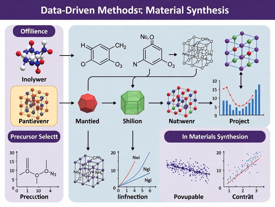
Data-Driven Synthesis of Single-Atom Catalysts
A compelling example of data-driven materials development is the recent work on single-atom catalysts (SACs) for water purification. Researchers employed a strategy combining data-driven predictions with precise synthesis to accelerate the development of high-performance SACs [4]. The process began with computational screening of 43 metal-N4 structures comprising transition and main group metal elements using a hard-template method [4].
The data-driven approach identified an iron-based single-atom catalyst (Fe-SAC) as the most promising candidate. This Fe-SAC featured a high loading of Fe-pyridine-N4 sites (approximately 3.83 wt%) and a highly mesoporous structure [4]. Experimental validation confirmed its exceptional performance, demonstrating an ultra-high decontamination performance with a rate constant of 100.97 minâ»Â¹ gâ»Â² [4]. The optimized Fe-SAC maintained continuous operation for 100 hours, representing one of the best performances reported for Fenton-like catalysts used in wastewater purification [4].
Table 2: Performance Metrics of Data-Driven Single-Atom Catalyst for Water Purification
| Parameter | Value | Significance |
|---|---|---|
| Fe-pyridine-N4 Site Loading | 3.83 wt% | High density of active sites |
| Rate Constant | 100.97 minâ»Â¹ gâ»Â² | Exceptional catalytic activity |
| Operational Stability | 100 hours | Practical durability for applications |
| Metal Structures Screened | 43 | Comprehensive computational selection |
| Key Mechanism | Selective singlet oxygen generation | Efficient pollutant degradation |
Experimental Protocols and Methodologies
Template-Based Synthesis Methods
The template method represents a powerful approach for controlling material morphology and pore structure during synthesis. This method involves using a template to direct the formation of target materials with precise structural characteristics [19]. The template method is simple, highly reproducible, and predictable, providing exceptional control over pore structure, dimensions, and material morphology [19].
The general synthesis procedure using templates includes three main steps: (1) preparation of templates, (2) synthesis of target materials using the templates, and (3) removal of templates [19]. Templates are classified based on their properties and spatial domain-limiting capabilities, with the most common classification distinguishing between hard templates and soft templates [19].
Hard Template Method
Hard templates typically consist of rigid materials with well-defined structures, such as porous silica, molecular sieves, metals, or carbons [19]. The synthesis process involves infiltrating the template with a precursor material, converting the precursor to a solid through chemical or thermal treatment, and subsequently removing the template through chemical etching or calcination [19]. Hard templates provide excellent domain limitation and high stability, enabling precise control over material size and morphology [19]. However, template removal can be challenging and may potentially damage the synthesized material structure [19].
Soft Template Method
Soft templates typically consist of surfactant molecules, polymers, or biological macromolecules that self-assemble into defined structures [19]. The synthesis occurs at the interface between the soft template and precursor materials, with molecular organization driven by micelle formation and intermolecular forces [19]. Soft templates generally offer milder removal conditions and simpler processing compared to hard templates, representing a current trend in template-based material preparation [19].
Protocol: Hydrothermal Synthesis of α-Fe₂O₃ Nanorod Template
The following detailed protocol exemplifies the synthesis of a specific template material used in various applications, including catalyst supports and functional materials:
Reagent Preparation:
- Dissolve 3.028 g of iron chloride hexahydrate (FeCl₃·6H₂O) and 0.72 g of urea (CO(NH₂)₂) in deionized water to form a 60 mL mixture solution [20].
Substrate Placement:
- Lean F-doped tin oxide (FTO) substrates perpendicularly in the reaction solution [20].
Hydrothermal Reaction:
- Seal the reaction vessel tightly and maintain at 100°C for 24 hours in an electric oven [20].
Annealing Treatment:
- Anneal the resulting products at 500°C for 30 minutes in a muffle furnace [20].
This protocol produces an α-Fe₂O₃ nanorod template suitable for further functionalization or use as a sacrificial template in subsequent material synthesis steps.
Data-Driven Catalyst Development Protocol
The development of high-performance single-atom catalysts follows a systematic data-driven protocol:
Computational Screening:
Candidate Selection:
- Identify promising candidates based on computational predictions, particularly focusing on structures that reduce energy barriers for key reaction steps [4].
Precise Synthesis:
- Employ hard-template methods to synthesize selected candidates with controlled atomic dispersion and porous structure [4].
Experimental Validation:
Mechanistic Study:
- Use computational methods to understand the fundamental mechanisms responsible for observed performance [4].
- For the Fe-SAC example, DFT calculations revealed that the catalyst reduced the energy barrier for intermediate O* formation, resulting in highly selective generation of singlet oxygen for pollutant degradation [4].
The Scientist's Toolkit: Research Reagent Solutions
Table 3: Essential Research Reagents for Template-Based Material Synthesis
| Reagent/Category | Function | Examples/Specific Instances |
|---|---|---|
| Hard Templates | Provide rigid scaffolding with controlled porosity for material synthesis | Porous silica, Mesoporous carbon, Metal oxides, Molecular sieves [19] |
| Soft Templates | Self-assembling molecular systems that direct material morphology | Surfactants, Polymers, Biological macromolecules [19] |
| Metal Precursors | Source of metallic components in catalyst synthesis | Iron chloride hexahydrate (FeCl₃·6H₂O), Zinc nitrate hexahydrate (Zn(NO₃)₂) [20] |
| Structure-Directing Agents | Control molecular organization during synthesis | Urea (CO(NHâ‚‚)â‚‚), Hexamethylenetetramine (C₆Hâ‚â‚‚Nâ‚„) [20] |
| Computational Resources | Enable prediction and screening of material properties | Density Functional Theory (DFT) codes, Materials databases (e.g., Digital Catalysis Platform) [4] [1] |
| Manifaxine | Manifaxine, CAS:135306-42-2, MF:C12H15F2NO2, MW:243.25 g/mol | Chemical Reagent |
| [Mpa1, D-Tic7]OT | [Mpa1, D-Tic7]OT|Oxytocin Analogue|RUO | [Mpa1, D-Tic7]OT is a synthetic oxytocin receptor modulator for research. This product is for Research Use Only, not for human or veterinary use. |
Integrated Workflows in the Materials Innovation Ecosystem
The full power of the materials innovation ecosystem emerges when stakeholders and methodologies integrate into cohesive workflows. The following diagram illustrates how data-driven approaches connect different elements of the ecosystem to accelerate materials development:
This integrated workflow demonstrates how data flows between stakeholders and methodology components, creating a virtuous cycle of prediction, synthesis, validation, and knowledge capture that accelerates materials innovation.
The Materials Innovation Ecosystem represents a paradigm shift in how materials are discovered, developed, and deployed. By fostering collaboration between academia, industry, and government stakeholders, and leveraging data-driven methodologies, this ecosystem dramatically accelerates the materials development timeline. Template-based synthesis methods provide precise control over material structure, while computational guidance and machine learning optimize experimental approaches and predict outcomes before laboratory work begins. As these methodologies continue to evolve and integrate, they promise to address pressing global challenges in areas such as water purification, sustainable energy, and advanced manufacturing through more efficient and targeted materials development.
A Toolbox for Innovation: Core Data-Driven Methods and Their Applications
In the competitive landscapes of materials science and pharmaceutical development, the conventional "one-variable-at-a-time" (OVAT) approach to experimentation has become a significant bottleneck. This trial-and-error method is not only time-consuming and resource-intensive but also frequently fails to identify optimal conditions because it cannot detect critical interactions between factors [6]. In response to these challenges, Design of Experiments (DoE) and Response Surface Methodology (RSM) have emerged as statistical powerhouses that enable researchers to systematically explore complex experimental spaces, model relationships between variables, and efficiently identify optimum conditions [21] [22].
The significance of these methodologies is particularly pronounced within the context of data-driven material synthesis research, where the parameter space is often large and multidimensional. Factors such as reagent choices, synthesis methods, temperature, time, stoichiometric ratios, and concentrations can interact in complex ways that defy conventional chemical intuition [6]. Similarly, in pharmaceutical formulation development, excipient combinations and processing parameters must be optimized to achieve critical quality attributes [23] [24]. DoE and RSM provide structured frameworks for navigating these complexities, transforming the experimental process from random exploration to targeted investigation.
Theoretical Foundations: Understanding DoE and RSM
Design of Experiments (DoE)
DoE is a systematic approach for planning, conducting, analyzing, and interpreting controlled tests to evaluate the factors that control the value of a parameter or group of parameters [25]. At its core, DoE involves the deliberate simultaneous variation of input factors (independent variables) to determine their effect on response variables (dependent variables) [25]. This approach allows researchers to maximize the information gained from a minimal number of experimental runs while ensuring statistical reliability.
Key principles underlying DoE include:
- Randomization: The random sequence of experimental runs to minimize the effects of lurking variables
- Replication: Repeated experimental runs to estimate variability and improve precision
- Blocking: Arranging experiments into homogeneous groups to account for known sources of variability
The advantages of DoE over OVAT approaches are substantial. While OVAT methods can only explore one-dimensional slices of a multidimensional parameter space, DoE captures interaction effects between factors—a critical capability since many material synthesis and pharmaceutical processes are driven by these interactions [6]. Furthermore, properly designed experiments can provide a prediction equation for the process in the form of Y = f(Xâ‚, Xâ‚‚, X₃...Xâ‚™), enabling researchers to forecast outcomes for untested factor combinations [25].
Response Surface Methodology (RSM)
RSM is a collection of mathematical and statistical techniques that builds upon DoE principles to model, analyze, and optimize processes where the response of interest is influenced by several variables [21] [22]. First introduced by Box and Wilson in 1951, RSM focuses on designing experiments, fitting mathematical models to empirical data, and exploring the relationships between multiple explanatory variables and one or more response variables [21] [22].
The methodology typically proceeds through sequential phases:
- Screening experiments to identify significant factors
- Steepest ascent/descent experiments to move rapidly toward the optimum region
- Detailed modeling using response surface designs to characterize the optimum region
RSM employs empirical model-fitting, most commonly using first-order or second-order polynomial functions. A standard quadratic RSM model is expressed as: Y = β₀ + ∑βᵢXᵢ + ∑βᵢᵢXᵢ² + ∑βᵢⱼXᵢXⱼ + ε where Y is the predicted response, β₀ is the constant coefficient, βᵢ represents the linear coefficients, βᵢᵢ represents the quadratic coefficients, βᵢⱼ represents the interaction coefficients, and ε is the random error term [21].
This empirical approach is particularly valuable when theoretical models of the process are cumbersome, time-consuming, inefficient, or unreliable [22]. By using a sequence of designed experiments, RSM enables researchers to locate optimal conditions—whether for maximizing, minimizing, or attaining a specific target for the response variable(s) [22].
Comparative Analysis: DoE versus Machine Learning
While both DoE/RSM and machine learning (ML) are data-driven approaches, they offer complementary strengths for different research scenarios. DoE is particularly advantageous for novel, low-throughput exploratory research where little prior knowledge exists and the ability to collect large datasets is limited [6]. Its regression-based analysis makes it ideally suited for continuous outcomes such as yield, particle size, or emission wavelength within a specific material phase [6].
In contrast, ML techniques typically require larger datasets but excel at mapping complex synthesis-structure-property relationships that may be beyond human intuition [6] [26]. ML classifiers can handle both mixed and categorical variables and outcomes, making them better suited for problems involving synthesis across multiple crystal phases or when high-throughput synthesis generates substantial data [6]. The integration of automated robotic systems and multichannel flow reactors with ML approaches has created powerful platforms for systematic exploration of synthetic landscapes [6].
Table 1: Comparison of DoE/RSM and Machine Learning Approaches
| Aspect | DoE/RSM | Machine Learning |
|---|---|---|
| Data Requirements | Effective with small datasets | Typically requires large datasets |
| Variable Types | Best with continuous variables | Handles mixed and categorical variables well |
| Primary Applications | Optimization within a known experimental region | Exploration of complex, high-dimensional spaces |
| Outcome Types | Continuous responses | Continuous and categorical outcomes |
| Experimental Bias | More susceptible to initial experimental region selection | Can uncover patterns beyond initial assumptions |
| Implementation Context | Low-throughput, novel systems | High-throughput, data-rich environments |
Experimental Design Strategies and Mathematical Frameworks
Key Experimental Designs in RSM
Central Composite Design (CCD)
Central Composite Design is one of the most prevalent response surface designs, consisting of three distinct components [21]:
- Factorial points: Represent all combinations of factor levels (as in a standard factorial design)
- Center points: Repeated runs at the midpoint of the experimental region to estimate experimental error and check model adequacy
- Axial points (star points): Positioned along each factor axis at a distance α from the center to capture curvature and enable estimation of quadratic effects
CCDs can be arranged in different variations including circumscribed CCD (axial points outside factorial cube), inscribed CCD (factorial points scaled within axial range), and face-centered CCD (axial points on factorial cube faces) [21]. A key property of CCDs is rotatability—the variance of predicted responses remains constant at points equidistant from the center, ensuring uniform precision across the experimental region [21] [22].
Box-Behnken Design (BBD)
Box-Behnken Designs are spherical, rotatable second-order designs based on balanced incomplete block designs [21] [24]. For a 3-factor BBD with one center point, the number of required runs is calculated as 2k × (k - 1) + nₚ, where k is the number of factors and nₚ is the number of center points [21]. This results in 13 runs for a 3-factor design [21].
BBDs are particularly advantageous when a full factorial experiment is impractical due to resource constraints, as they efficiently explore the factor space with fewer experimental runs than a full factorial design [21] [27]. However, they do not include corner points and are therefore inappropriate when testing at extreme factor settings is necessary.
Table 2: Comparison of Primary RSM Experimental Designs
| Design Characteristic | Central Composite Design (CCD) | Box-Behnken Design (BBD) |
|---|---|---|
| Design Points | Factorial + Center + Axial points | Combinations of midpoints of factor edges + center points |
| Number of Runs (3 factors) | 15-20 depending on center points | 13 |
| Factor Levels | 5 levels | 3 levels |
| Region of Interest | Cuboidal or spherical | Spherical |
| Applications | Sequential experimentation | When extreme conditions are undesirable |
| Advantages | Can be used sequentially; estimates curvature well | Fewer runs than CCD; avoids extreme factor combinations |
Model Fitting and Analysis
Once experimental data are collected according to the designed matrix, the next critical step is fitting a mathematical model that describes the relationship between factors and responses [21]. Regression analysis, typically via least squares method, is used to estimate coefficients (β₀, βᵢ, βᵢⱼ) in the polynomial equation [21].
The validity and significance of the fitted model are then evaluated using Analysis of Variance (ANOVA), which decomposes the total variability in the data into components attributable to each factor, their interactions, and residual error [27] [25]. Key metrics in model evaluation include:
- Coefficient of Determination (R²): Proportion of variance in the response explained by the model
- Adjusted R²: R² adjusted for the number of terms in the model
- Predicted R²: Measure of how well the model predicts new data
- p-values: Statistical significance of model terms
Model adequacy is further checked through diagnostic plots of residuals, which should be independent, normally distributed, and have constant variance [25].
Application Protocols: Materials Synthesis and Pharmaceutical Development
Protocol 1: Optimizing Inorganic Material Synthesis Using DoE/RSM
Background: The synthesis of novel inorganic materials with tailored properties represents a significant challenge in materials science. Traditional OVAT approaches often fail to identify true optima due to complex interactions between synthesis parameters [6].
Objective: To systematically optimize the synthesis of an inorganic material (e.g., metal oxide nanoparticles) for target properties such as particle size, yield, and crystallinity.
Experimental Workflow:
Step-by-Step Procedure:
Define Objective and Responses: Clearly articulate the research goal—e.g., "minimize particle size while maximizing yield of metal oxide nanoparticles." Identify measurable responses (e.g., particle size, PDI, yield, crystallite size) and establish measurement protocols [6].
Identify Critical Factors: Through literature review and preliminary experiments, identify key process parameters likely to influence responses. Common factors in inorganic synthesis include:
- Precursor concentration
- Temperature and time
- pH
- Mixing rate
- Reactant stoichiometry
Select Experimental Design: Begin with a screening design (e.g., fractional factorial) if many factors are being considered. For detailed optimization with limited factors (typically 2-5), employ RSM designs such as CCD or BBD. Determine factor levels based on practical constraints and preliminary knowledge [6] [21].
Execute Experimental Runs: Perform synthesis according to the randomized run order specified by the design matrix. Maintain careful control over non-studied parameters. Document any unexpected observations or deviations from protocol.
Analyze Data and Fit Model: Use statistical software to:
- Perform ANOVA to identify significant factors and interactions
- Fit an appropriate model (linear, quadratic, or special cubic)
- Check model adequacy through residual analysis
- Generate contour and 3D surface plots to visualize factor-response relationships [21]
Validate Model and Optimize: Conduct confirmation experiments at predicted optimal conditions. Compare predicted versus actual responses to validate model accuracy. If discrepancy exceeds acceptable limits, consider model refinement through additional experiments [6].
Research Reagent Solutions for Inorganic Material Synthesis:
- Metal Salt Precursors: Source of metal ions (e.g., metal nitrates, chlorides, acetylacetonates); purity >99% recommended
- Precipitation Agents: Hydroxides, carbonates, or organic precipitants that control nucleation and growth
- Surfactants/Templating Agents: Structure-directing agents (e.g., CTAB, PVP) to control particle size and morphology
- Solvents: High-purity aqueous and non-aqueous media with controlled ionic strength and pH
- Dopants: Trace elements for modifying material properties, typically 0.1-5 mol%
Protocol 2: Pharmaceutical Formulation Optimization Using RSM
Background: Pharmaceutical formulation development requires balancing multiple, often competing, quality attributes. The case study of levetiracetam effervescent tablets demonstrates RSM's applicability to pharmaceutical systems [24].
Objective: To optimize an effervescent tablet formulation containing citric acid (Xâ‚: 320-960 mg) and effersoda (Xâ‚‚: 320-960 mg) to achieve target effervescence time, hardness, and friability [24].
Experimental Workflow:
Step-by-Step Procedure:
Define Critical Quality Attributes (CQAs) and Critical Process Parameters (CPPs): Identify formulation and process parameters with significant impact on product quality. For effervescent tablets, key factors include acid:base ratio, compression force, and lubricant concentration [24].
Select RSM Design: For two factors, a Central Composite Rotatable Design (CCRD) with 14 runs (6 center points, 4 cube points, 4 axial points) provides efficient exploration of the design space while allowing estimation of quadratic effects [24].
Prepare Tablet Batches: Manufacture tablets according to the experimental design using appropriate processing methods (e.g., dry granulation via roll compaction for moisture-sensitive formulations) [24].
Characterize Tablets: Evaluate CQAs for each batch including:
- Effervescence time (target: complete dissolution within 3-5 minutes)
- Tablet hardness (using pharmaceutical hardness tester)
- Friability (using Roche friabilator)
- Drug content uniformity [24]
Develop Polynomial Models: Fit second-order polynomial models to each response using multiple linear regression. For the levetiracetam case study, the models demonstrated excellent correlation with R² values of 0.9808, 0.9939, and 0.9892 for effervescence time, hardness, and friability, respectively [24].
Apply Desirability Function for Multi-Response Optimization: Use desirability functions to simultaneously optimize multiple responses. Transform each response to a desirability value (0-1 scale), then calculate overall desirability as the geometric mean of individual desirabilities [24].
Research Reagent Solutions for Pharmaceutical Formulation:
- API (Active Pharmaceutical Ingredient): Drug substance (e.g., levetiracetam, bisoprolol fumarate) with specified purity and particle size distribution
- Effervescent Couple: Acid (citric, tartaric, adipic) and base (sodium bicarbonate, sodium carbonate, effersoda) components in optimal ratio
- Binders/Diluents: Water-soluble excipients (mannitol, sorbitol, anhydrous lactose) for tablet structure and dissolution
- Lubricants: Magnesium stearate, sodium stearyl fumarate in minimal concentrations (0.5-2%) to prevent sticking
- Sweeteners/Flavors: Aspartame, acesulfame-K, and pharma-approved flavors to enhance palatability
Validation and Performance Metrics: Case Study in Hybrid Materials
Background: A comprehensive 2024 study compared the effectiveness of factorial, Taguchi, and RSM models for analyzing mechanical properties of epoxy matrix composites reinforced with natural Chambira fiber and synthetic fibers [28].
Experimental Design: The research employed 90 treatments with three replicates for each study variable, creating a robust dataset for model validation [28].
Performance Outcomes:
Table 3: Model Performance Comparison for Hybrid Material Analysis [28]
| Statistical Model | Coefficient of Determination (R²) | Predictive Capability | Overall Desirability | Key Findings |
|---|---|---|---|---|
| Modified Factorial | >90% for most mechanical properties | High | 0.7537 | Best suited for research with 99.73% overall contribution |
| Taguchi | Variable across properties | Moderate | Not specified | Effective for initial screening |
| RSM | Strong for specific responses | High for targeted optimization | Not specified | Excellent for mapping response surfaces |
The validation study revealed that model refinement by considering only significant source elements dramatically improved performance metrics, reflected in increased coefficients of determination and enhanced predictive capacity [28]. The modified factorial model emerged as most appropriate for this materials research application, achieving an overall contribution of 99.73% with global desirability of 0.7537 [28].
Advanced Applications and Integration with Emerging Technologies
The integration of DoE/RSM with other analytical and computational methods creates powerful frameworks for complex research challenges. A notable example comes from polymer nanocomposites, where researchers combined DoE, RSM, and Partial Least Squares (PLS) regression to characterize and optimize low-density polyethylene/organically modified montmorillonite nanocomposites [29].
This integrated chemometric approach enabled simultaneous correlation of four processing parameters (clay concentration, compatibilizer concentration, mixing temperature, and mixing time) with six nanocomposite properties (interlayer distance, decomposition temperature, melting temperature, Young's modulus, loss modulus, and storage modulus) [29]. The PLS model achieved an R² of 0.768 (p ≤ 0.05), identifying clay% and compatibilizer% as the most influential parameters while revealing complex interactions among factors [29].
Looking forward, the convergence of traditional statistical methods with artificial intelligence and automation presents exciting opportunities. Machine learning algorithms can enhance DoE/RSM by:
- Identifying complex nonlinear relationships beyond polynomial approximations
- Optimizing experimental designs for specific objectives
- Enabling real-time adaptive experimentation through robotic platforms
- Facilitating knowledge transfer between related material systems [26]
These advanced applications highlight how DoE and RSM continue to evolve as foundational methodologies within the broader context of data-driven research, maintaining their relevance through integration with emerging technologies rather than being replaced by them.
The adoption of machine learning (ML) for property prediction represents a paradigm shift in materials science and drug discovery, enabling the rapid identification of novel materials and compounds with tailored characteristics. This shift is propelled by the convergence of increased computational power, the proliferation of experimental and computational data, and advancements in ML algorithms [30]. Data-driven science is now recognized as the fourth scientific era, complementing traditional experimental, theoretical, and computational research methods [30]. This article provides detailed application notes and protocols for applying ML to property prediction, framed within the broader context of data-driven methods for material synthesis research. We focus on the evolution from classical supervised learning to sophisticated deep neural networks, with a particular emphasis on overcoming the pervasive challenge of data scarcity. The protocols herein are designed for an audience of researchers, scientists, and drug development professionals seeking to implement these powerful techniques.
Technical Approaches and Comparative Analysis
The selection of an appropriate ML strategy is contingent upon the specific prediction task, the nature of the available data, and the molecular representation. The following section compares the predominant technical frameworks.
# Table 1: Comparison of ML Approaches for Property Prediction
| Approach | Core Principle | Key Advantages | Ideal Use Case | Representative Performance |
|---|---|---|---|---|
| Quantitative Structure-Property Relationship (QSPR) | Correlates hand-crafted molecular descriptors or fingerprints with a target property using statistical or ML models [31] [32]. | High interpretability; Lower computational cost; Effective with small datasets [31]. | Rapid prototyping and prediction for small organic molecules when data is limited [31]. | Inclusion of MD descriptors improves prediction, especially with <1000 data points [31]. |
| Graph Neural Networks (GNNs) | End-to-end learning directly from graph representations of molecules (atoms as nodes, bonds as edges) [33] [31]. | Eliminates need for manual descriptor selection; Automatically learns relevant features [33]. | Capturing complex structure-property relationships in polymers and molecules with sufficient data [33]. | State-of-the-art for many molecular tasks; RMSE reduced by 28.39% for electron affinity with SSL [33]. |
| Self-Supervised Learning (SSL) with GNNs | Pre-trains GNNs on pseudo-tasks derived from unlabeled molecular graphs before fine-tuning on the target property [33]. | Dramatically reduces required labeled data; Learns universal structural features [33]. | Polymer and molecular property prediction in scarce labeled data domains [33]. | Decreases RMSE by 19.09-28.39% in scarce data scenarios vs. supervised GNNs [33]. |
| Physics-Informed Machine Learning | Integrates physics-based descriptors or constraints (e.g., from MD simulations) into ML models [31]. | Improved accuracy and interpretability; Leverages domain knowledge; Better generalization [31]. | Predicting properties like viscosity where intermolecular interactions are critical [31]. | QSPR models with MD descriptors reveal intermolecular interactions as most important for viscosity [31]. |
| Multi-Task Learning (MTL) | Simultaneously trains a single model on multiple related prediction tasks [34]. | Improved generalization by leveraging shared information across tasks; More efficient data use [34]. | Predicting multiple ADME properties for drugs or related material properties concurrently [34]. | Enables modeling of 25 ADME endpoints with shared representations; comparable performance for TPDs [34]. |
Detailed Experimental Protocols
Protocol 1: Self-Supervised GNNs for Polymer Property Prediction
This protocol adapts the methodology from Gao et al. for predicting polymer properties like electron affinity and ionization potential with limited labeled data [33].
1. Polymer Graph Representation:
- Objective: Convert a polymer structure into a stochastic graph representation.
- Steps:
- Represent each atom as a node and each bond as a pair of directed edges.
- Assign feature vectors to each node (atom type, etc.) and each directed edge.
- Incorporate stochastic weights on nodes and edges to represent features like monomer stoichiometry and chain architecture [33].
- Software: Implement using deep learning frameworks (PyTorch, TensorFlow) with cheminformatics libraries.
2. Self-Supervised Pre-training:
- Objective: Pre-train a GNN model to learn fundamental polymer structural features without property labels.
- Methods (to be used ensemble):
- Model Architecture: Use a Weighted Directed Message Passing Neural Network tailored for the polymer graph representation [33].
3. Supervised Fine-tuning:
- Objective: Adapt the pre-trained model to the specific target property prediction task.
- Steps:
- Replace the pre-training output layers with a new regression (or classification) head for the target property.
- Initialize the GNN layers with the pre-trained weights.
- Train the entire model on the small, labeled dataset using a standard regression loss (e.g., Mean Squared Error).
- Transfer Strategy: The best performance is achieved with an ensemble of node-, edge-, and graph-level pre-training and transferring all GNN layers [33].
Protocol 2: Physics-Informed QSPR for Viscosity Prediction
This protocol is based on the work for predicting temperature-dependent viscosity of small organic molecules [31].
1. Data Curation and Preprocessing:
- Data Collection: Curate experimental viscosity data with associated temperatures and SMILES strings from literature and databases.
- Data Filtering:
- Filter for specific atomic elements and remove stereoisomers if minimal.
- Apply outlier detection (e.g., box-and-whisker plot method) to remove extreme values of viscosity and temperature.
- Remove data points that violate the inverse relationship between viscosity and temperature [31].
- Data Transformation: Apply a log-transform to the viscosity values (log μ) to correct for data skew [31].
2. Feature Engineering:
- Molecular Descriptors: Generate 209 RDKit descriptors, 1000-bit Morgan fingerprints, and 132 Matminer descriptors.
- Preprocess by removing correlated features (Pearson’s r ≥ 0.90) and constant features, then standardize the remaining features [31].
- Physics-Informed Descriptors: Incorporate descriptors derived from Molecular Dynamics (MD) simulations, such as those capturing intermolecular interactions [31].
- External Variable: Include the inverse of temperature (1/T) as an input feature, reflecting the empirical Vogel equation [31].
3. Model Training and Evaluation:
- Algorithm Selection: Train and benchmark multiple algorithms, including Multilayer Perceptron (MLP), Support Vector Regression (SVR), Random Forest (RF), and Gradient Boosting methods (GBR, LGBM, XGBoost) [31].
- Validation: Use rigorous validation schemes like k-fold cross-validation or temporal hold-out to ensure model generalizability.
- Interpretation: Use feature importance tools (e.g., SHAP) to identify key molecular and MD descriptors, validating the model against physical understanding [31].
Workflow Visualization
# Polymer Property Prediction with Self-Supervised GNNs
# Physics-Informed QSPR Workflow
The Scientist's Toolkit
# Table 2: Essential Research Reagents and Software Solutions
| Tool / Resource | Type | Primary Function | Application Example |
|---|---|---|---|
| QSPRpred | Software Package | A flexible, open-source Python toolkit for building, benchmarking, and deploying QSPR models with high reproducibility [32]. | Streamlines the entire QSPR workflow from data preparation to model deployment, supporting multi-task learning [32]. |
| Polymer Graph Representation | Data Structure | A stochastic graph that encodes monomer combinations, chain architecture, and stoichiometry for ML readiness [33]. | Enables the application of GNNs to polymer systems by providing a meaningful input representation [33]. |
| RDKit | Cheminformatics Library | Generates molecular descriptors (209), fingerprints, and processes SMILES strings [31]. | Used in feature engineering for traditional QSPR models to convert structures into numerical vectors [31]. |
| MD Simulation Descriptors | Physics-Informed Feature | Descriptors derived from molecular dynamics simulations that capture intermolecular interactions [31]. | Informs ML models of physical principles, improving accuracy for properties like viscosity [31]. |
| DeepChem | Deep Learning Library | Provides a wide array of featurizers and graph-based models for molecular property prediction [32]. | Rapid prototyping of GNN and other deep learning models on molecular datasets. |
| Multi-Task Global Models | Modeling Strategy | An ensemble of message-passing neural networks and DNNs trained on multiple ADME endpoints simultaneously [34]. | Predicts a suite of pharmacokinetic properties (e.g., permeability, clearance) for novel drug modalities [34]. |
| Xenyhexenic Acid | Xenyhexenic Acid|266.3 g/mol | Bench Chemicals | |
| Abx-002 | ABX-002 / Qtw4WC4brx | ABX-002 (Qtw4WC4brx) is an investigational FAAH-activated prodrug for research. This product is for Research Use Only (RUO), not for human or veterinary use. | Bench Chemicals |
The integration of machine learning into property prediction is fundamentally accelerating the design cycles for new materials and therapeutic agents. As detailed in these application notes, the field is moving beyond simple supervised learning on hand-crafted features toward sophisticated, end-to-end deep learning models. Critical to this evolution are strategies like self-supervised learning and physics-informed ML, which directly address the industry-wide challenge of data scarcity. The provided protocols, workflows, and toolkit offer a practical foundation for researchers to implement these advanced methods. The future of data-driven material synthesis lies in the continued development of robust, generalizable models that seamlessly integrate domain knowledge, thereby closing the loop between predictive in-silico screening and experimental realization.
Inverse design represents a paradigm shift in materials discovery, moving from traditional trial-and-error approaches to a targeted, property-driven methodology. Unlike conventional forward design that predicts material properties from a known structure or composition (ACS - Atomic constituents, Composition, and Structure), inverse design starts with a desired property or functionality as the input and identifies the material that fulfills it [35] [36]. This approach is particularly powerful for addressing society's pressing technological needs, such as developing materials for more efficient energy storage, superior catalysts, or sustainable packaging, where the ideal material is unknown but the performance requirements are clearly defined [37] [36].
This property-to-structure inversion is made possible by deep generative models, a class of artificial intelligence that learns the complex relationships between material structures and their properties from existing data. Once trained, these models can navigate the vast chemical space to generate novel, viable material candidates that are optimized for specific target properties [37] [38]. The application of this methodology is accelerating innovation across diverse domains, including the design of inorganic functional materials, catalysts, and sustainable food packaging [37] [39] [40].
Core Methodologies and Generative Models
The implementation of inverse design relies on several key machine learning architectures, each with distinct strengths for different aspects of the materials generation problem.
Generative Adversarial Networks (GANs)
Generative Adversarial Networks (GANs) consist of two competing neural networks: a generator that creates candidate materials and a discriminator that evaluates them against real data. This adversarial training process pushes the generator to produce increasingly realistic and stable structures [39]. Their application is particularly noted in designing sustainable food packaging materials, where a GAN-based framework successfully generated over 100 theoretically viable candidates, with 20% exhibiting superior barrier and degradation properties [39]. The conditional GAN (cGAN) variant is especially valuable for inverse design, as it allows the generation of materials conditioned on specific property targets [39].
Variational Autoencoders (VAEs)
Variational Autoencoders (VAEs) learn a compressed, continuous latent representation of material structures. This latent space can be intelligently navigated or sampled to generate new structures with desired characteristics [37]. A key advancement is the integration of VAEs with topological descriptors, which enhances the interpretability of the design process. For instance, a team used a topology-based VAE to inversely design catalytic active sites, uncovering a strong linear correlation between topological invariants (Betti numbers) and adsorption energies, thereby providing physical insight into the structure-property relationship [40].
Diffusion Models
Diffusion models generate data by iteratively refining noise into a structured output, a process that has recently been adapted for crystalline materials. MatterGen is a state-of-the-art, diffusion-based model designed specifically for generating stable, diverse inorganic materials across the periodic table [38]. It introduces a customized diffusion process for atom types, coordinates, and the periodic lattice, and uses adapter modules for fine-tuning towards multiple property constraints. MatterGen more than doubles the percentage of generated stable, unique, and new (SUN) materials compared to previous models and produces structures that are more than ten times closer to their DFT-relaxed ground state [38].
Table 1: Comparison of Key Deep Generative Models for Inverse Design
| Model Type | Core Mechanism | Key Advantages | Example Applications |
|---|---|---|---|
| Generative Adversarial Network (GAN) | Adversarial training between generator and discriminator [39] | Capable of generating high-quality, realistic samples [39] | Sustainable packaging materials [39] |
| Variational Autoencoder (VAE) | Compresses data into a continuous latent space [37] | Enables smooth interpolation and exploration in latent space; can be combined with topological descriptors for interpretability [40] | Catalytic active sites, vanadium oxides [37] [40] |
| Diffusion Model | Iterative denoising from a noise prior [38] | High stability and diversity of generated materials; excels at multi-property optimization [38] | General inorganic materials design (MatterGen) [38] |
Quantitative Performance and Data
The effectiveness of inverse design models is quantified through their ability to propose novel, stable, and property-optimized materials with high computational efficiency.
The MatterGen model sets a new benchmark, with 78% of its generated structures calculated to be stable (within 0.1 eV/atom of the convex hull) using Density Functional Theory (DFT). Furthermore, 61% of its generated structures are entirely new, and it achieves an unprecedented structural quality, with 95% of generated structures having an atomic RMSD below 0.076 Ã… from their DFT-relaxed forms [38]. In a specialized application for sustainable packaging, a GAN-based framework demonstrated a 20-100x acceleration in screening efficiency compared to traditional DFT calculations while maintaining high accuracy [39]. For catalytic design, a topology-based VAE achieved a remarkably low mean absolute error of 0.045 eV for predicting *OH adsorption energy, despite being trained on a relatively small dataset of around 1,100 samples [40].
Table 2: Key Performance Metrics from Recent Inverse Design Studies
| Study / Model | Primary Metric | Reported Performance | Implication for Materials Discovery |
|---|---|---|---|
| MatterGen (Diffusion) [38] | Stability (within 0.1 eV/atom of convex hull) | 78% | Vast majority of generated candidates are theoretically stable. |
| MatterGen (Diffusion) [38] | Novelty (not in training databases) | 61% | Model explores new chemical space beyond known materials. |
| MatterGen (Diffusion) [38] | Structural Relaxation RMSD | < 0.076 Ã… (95% of samples) | Generated structures are very close to their local energy minimum. |
| GAN (Packaging) [39] | Screening Acceleration | 20-100x faster than DFT | Dramatically reduces computational cost and time. |
| Topological VAE (Catalysis) [40] | Adsorption Energy MAE | 0.045 eV | High predictive accuracy even with limited data. |
Application Notes and Experimental Protocols
This section provides a detailed workflow and protocol for implementing an inverse design pipeline for material synthesis, from computational generation to experimental validation.
Workflow for Inverse Design and Synthesis
The following diagram outlines the core cyclical workflow of inverse design, integrating computational generation with experimental validation.
Protocol 1: Model Training and Candidate Generation
This protocol covers the initial computational phase of the inverse design process.
4.2.1 Define Property Constraints and Data Sourcing
- Objective: Establish clear, quantifiable target properties (e.g., band gap > 1.5 eV, specific magnetic moment, low supply-chain risk composition) [38].
- Procedure: Curate a training dataset from large-scale materials databases such as the Materials Project, OQMD, or OMat24 [39] [38]. For the OMat24 dataset, which contains 110 million DFT-calculated structures, extract relevant material subsystems and their corresponding properties [39].
4.2.2 Model Selection and Configuration
- Objective: Choose a generative model architecture suited to the problem.
- Procedure:
- Configuration: Implement a property prediction network, such as an enhanced EquiformerV2 graph neural network, to guide the generation. This network should be trained to predict key properties like formation energy, with a target Mean Absolute Error (MAE) of ~12 meV/atom or lower [39].
4.2.3 Generation and Computational Screening
- Objective: Produce and filter candidate materials.
- Procedure:
- Generate a large batch of candidate structures (e.g., 10,000-1,000,000) using the trained model [38].
- Employ a computational funnel: First, use fast machine learning predictors to filter for stability. Then, perform more accurate but costly DFT calculations on the shortlisted candidates to verify stability (e.g., energy above convex hull < 0.1 eV/atom) and calculate target properties [39] [38].
- Select the top 10-50 candidates that best meet the target properties and show good thermodynamic stability for experimental synthesis.
Protocol 2: Experimental Synthesis and Validation
This protocol outlines the steps for translating computationally generated candidates into real, characterized materials.
4.3.1 Synthesis Planning
- Objective: Devise a viable synthesis route for the predicted material.
- Procedure: Use calculated phase diagrams from databases to identify stable synthesis conditions and potential precursors [41]. For novel compositions, leverage high-throughput combinatorial synthesis approaches or panoramic synthesis to explore a range of conditions (temperature, pressure, precursor ratios) simultaneously [41].
4.3.2 In Situ Characterization
- Objective: Monitor the synthesis reaction in real-time to understand reaction pathways and intermediates.
- Procedure: Utilize in situ characterization techniques such as X-ray diffraction (XRD) or neutron scattering during synthesis. This provides critical feedback on phase formation and purity, helping to optimize synthesis parameters rapidly [41].
4.3.3 Ex Situ Characterization and Property Validation
- Objective: Confirm the structure and measure the final properties of the synthesized material.
- Procedure:
- Characterize the synthesized powder or crystal using XRD and compare the diffraction pattern with the computationally predicted structure [38].
- Use techniques like scanning electron microscopy (SEM) and energy-dispersive X-ray spectroscopy (EDS) to analyze morphology and composition.
- Perform functional property measurements relevant to the initial design goal (e.g., measure magnetic properties using a SQUID magnetometer, electronic properties using impedance spectroscopy, or barrier properties for packaging materials) [39] [38].
- The synthesis is considered successful if the experimentally measured property is within a pre-defined margin (e.g., 20%) of the target value [38].
Table 3: Key Computational and Experimental Resources for Inverse Design
| Resource Name | Type | Function in Inverse Design |
|---|---|---|
| OMat24 Dataset [39] | Computational Database | Provides 110 million DFT-calculated inorganic structures for training generative and property prediction models. |
| Materials Project [38] | Computational Database | A curated database of known and computed materials for data sourcing and stability assessment (convex hull). |
| EquiformerV2 [39] | Graph Neural Network | Accurately predicts formation energy and functional properties of generated candidates to guide the design process. |
| Persistent GLMY Homology (PGH) [40] | Topological Descriptor | Extracts interpretable, invariant features from atomic structures (e.g., connectivity, voids) to inform generative models. |
| Density Functional Theory (DFT) [39] | Computational Simulation | The gold-standard for final validation of candidate stability and electronic properties before synthesis. |
| In Situ XRD [41] | Experimental Characterization | Provides real-time, atomic-scale insight into phase formation and transformation during synthesis. |
High-Throughput Virtual Screening (HTVS) for Accelerated Candidate Discovery
High-Throughput Virtual Screening (HTVS) has emerged as a transformative computational methodology that leverages automation, data processing, and predictive modeling to rapidly evaluate extremely large libraries of chemical compounds or materials for desired properties. By simulating interactions and predicting performance in silico, HTVS enables researchers to prioritize the most promising candidates for further experimental validation, dramatically accelerating discovery timelines in both pharmaceutical and materials science research [42] [43]. This approach is particularly powerful within data-driven material synthesis frameworks, where it reduces reliance on traditional resource-intensive and time-consuming iterative physical experiments [44].
The paradigm has evolved significantly with advancements in computational power and machine learning (ML). Modern HTVS can process billions of compounds, leveraging techniques from molecular docking to sophisticated ML models that learn complex structure-property relationships [45] [43]. This shift towards digitized design, which integrates high-throughput computing (HTC) with intelligent algorithms, is revolutionizing discovery pipelines, making them faster, cheaper, and more efficient [44].
Key HTVS Protocols and Workflows
This section details the core experimental and computational protocols that form the foundation of a successful HTVS campaign.
General HTVS Workflow
A standard HTVS workflow involves several interconnected stages, from target definition to hit validation. The logical flow and dependencies between these stages are outlined in the diagram below.
Protocol 1: Ligand-Based Virtual Screening
Ligand-based screening is employed when the 3D structure of the target is unknown, but information about active compounds is available.
- Objective: To identify novel candidates in large chemical libraries that are structurally or physiochemically similar to known active molecules.
- Pre-processing Steps:
- Query Compound Curation: Collect a set of known active compounds (e.g., from databases like BindingDB) with confirmed activity against the target. Ensure data quality and consistency [45].
- Molecular Featurization: Encode the molecular structures of both query compounds and the screening library into numerical descriptors. Common descriptors include ECFP4 fingerprints, molecular weight, logP, and topological polar surface area [45].
- Screening Execution:
- Similarity Calculation: Compute the similarity between the query compounds and every molecule in the screening library. The Tanimoto coefficient is a standard metric for fingerprint-based similarity [45].
- Potency-Aware Embeddings: For advanced ML models, molecules are mapped into a continuous vector space using models like Transformers, pre-trained on large chemical databases (e.g., PubChem). Potency-aware embeddings can be generated by fine-tuning on specific activity data (e.g., from BindingDB) [45].
- High-Performance Search: Use optimized search algorithms (e.g., SIMD-optimized cosine similarity search over pre-indexed libraries) to rapidly identify nearest neighbors in the descriptor space [45].
- Post-processing:
- Hit Prioritization: Rank compounds based on similarity scores or proximity in the embedding space.
- Novelty Filtering: Apply filters to prioritize scaffolds distinct from known actives (e.g., ECFP4 Tanimoto ≤ 0.4) to enable scaffold hopping [45].
- Liability Filtering: Remove compounds with undesirable properties using filters like REOS (Rapid Elimination of Swill) and PAINS (Pan-Assay Interference Compounds) [45].
Protocol 2: Structure-Based Virtual Screening (Molecular Docking)
This protocol is used when the three-dimensional structure of the biological target (e.g., a protein) is available.
- Objective: To predict the binding pose and affinity of small molecules within a target's binding site.
- Pre-processing Steps:
- Protein Preparation: Obtain the 3D structure from a protein data bank (PDB). Add hydrogen atoms, assign protonation states, and remove water molecules unless critical for binding.
- Binding Site Definition: Define the spatial coordinates of the binding site, often based on the location of a co-crystallized ligand or known mutagenesis data.
- Ligand Library Preparation: Convert the compound library from 1D or 2D representations (like SMILES) into 3D structures. Generate plausible tautomers and stereoisomers.
- Screening Execution:
- Docking Simulation: For each compound in the library, the docking algorithm performs a conformational search to generate multiple poses within the binding site.
- Scoring: Each pose is scored using a scoring function that estimates the binding free energy. Common functions are based on force fields, empirical data, or knowledge-based potentials.
- Post-processing:
- Pose Analysis and Ranking: Visually inspect top-ranked poses for sensible interactions (e.g., hydrogen bonds, hydrophobic contacts) and rank compounds by their docking scores.
- Consensus Scoring: Improve robustness by combining results from multiple scoring functions.
- Interaction Fingerprinting: Analyze and compare the interaction patterns of top hits to known actives.
Protocol 3: Machine Learning-Guided HTVS for Materials Discovery
This protocol is tailored for discovering functional materials, such as emitters for OLEDs or energy materials.
- Objective: To rapidly screen vast chemical spaces for materials with target properties using predictive ML models and molecular descriptors.
- Pre-processing Steps:
- Descriptor Development: Identify or develop physically meaningful molecular descriptors that correlate with the target property. For instance, for inverted singlet-triplet (IST) fluorescence emitters, descriptors based on exchange integrals (
K_S) and orbital energy differences (O_D) have been shown to be highly effective [46]. - Data Set Curation: Assemble a training dataset of materials with known properties, often generated from high-throughput first-principles calculations (e.g., Density Functional Theory) [44] [47].
- Descriptor Development: Identify or develop physically meaningful molecular descriptors that correlate with the target property. For instance, for inverted singlet-triplet (IST) fluorescence emitters, descriptors based on exchange integrals (
- Screening Execution:
- Model Training: Train ML models—such as Graph Neural Networks (GNNs), Random Forest, or Gradient Boosting—on the curated dataset to learn the mapping from molecular structure or descriptors to the property of interest [44] [47].
- High-Throughput Prediction: Use the trained model to predict properties for every compound in a large virtual library (e.g., 3,486 molecules [46] or even billions [45]).
- Post-processing:
- Candidate Selection: Filter predictions based on performance thresholds (e.g., radiative decay rate
kr > 10^5 sâ»Â¹and photoluminescence quantum yieldPLQY > 0.6for OLED emitters [48]). - Accuracy Validation: Submit a subset of top candidates for accurate, computationally expensive validation (e.g., using post-Hartree-Fock methods like ADC(2) or experimental calibration) [48] [46].
- Candidate Selection: Filter predictions based on performance thresholds (e.g., radiative decay rate
Case Studies in Discovery
Case Study 1: Discovery of Phosphorescent Pt(II) Complexes for OLEDs
- Background: The development of organic light-emitting diodes (OLEDs) requires phosphorescent metal complexes with high radiative decay rate constants (
kr) and photoluminescence quantum yields (PLQY) [48]. - HTVS Application: Researchers implemented a multi-tiered protocol:
- Library Generation: Over 3,600 synthesis-friendly Pt(II) complex structures were generated [48].
- Machine Learning Screening: Three HTVS-ML models were built using carefully designed features for metal complexes to perform an initial screening [48].
- Accurate Prediction and Validation: 30 potential candidates identified by ML were subjected to highly accurate prediction using a Δ-learning method. This process confirmed 12 promising complexes with superior core structures. Experimental validation of two closely related complexes showed excellent emission properties, confirming the protocol's efficacy [48].
Table 1: Performance Metrics for Discovered Pt(II) Complexes [48]
| Metric | Screening Threshold | Confirmed Outcome |
|---|---|---|
Radiative Decay Rate Constant (k_r) |
> 10âµ sâ»Â¹ | Achieved in 12 promising complexes |
| Photoluminescence Quantum Yield (PLQY) | > 0.6 | Achieved in 12 promising complexes |
| Number of Initial Virtual Structures | 3,600+ | - |
| Number of Promising Complexes Identified | - | 12 |
Case Study 2: Ultra-High-Throughput Discovery of LRRK2 Inhibitors
- Background: Leucine-rich repeat kinase 2 (LRRK2) is a promising target for Parkinson's disease therapy [45].
- HTVS Application: The BIOPTIC B1 system was used for an ultra-HTS campaign:
- Scale: The system screened a 40-billion-compound library (Enamine REAL Space) [45].
- Technology: A SMILES-based Transformer model generated potency-aware embeddings for each molecule, and a high-speed search was performed over the pre-indexed library [45].
- Workflow: The campaign used diverse known inhibitors as queries, prioritized compounds with CNS-friendly properties and high novelty, and synthesized candidates via a partnered vendor [45].
- Results: The campaign resulted in the discovery of novel LRRK2 binders with sub-micromolar affinity (best Kd = 110 nM) in a matter of weeks, demonstrating a significant acceleration compared to traditional timelines [45].
Table 2: Key Outcomes from the LRRK2 Inhibitor Screening Campaign [45]
| Parameter | Value | Significance |
|---|---|---|
| Library Size | 40 billion compounds | Demonstrates ultra-HTS scale |
| Cycle Time | 11 weeks (synthesis to result) | Drastically reduced discovery time |
| Confirmed Binders | 14 | High success rate |
| Best Binding Affinity (Kd) | 110 nM | Sub-micromolar potency achieved |
| Hit Rate from Analog Expansion | 21% (10 actives from 47 analogs) | Validates scaffold and supports lead optimization |
Implementation Guide
A successful HTVS campaign relies on a suite of computational and data resources.
Table 3: Essential Tools and Resources for HTVS
| Category | Item | Function and Example |
|---|---|---|
| Computational Hardware | High-Performance Computing (HPC) / Cloud Computing | Provides the processing power for large-scale simulations and ML model training [43]. |
| Software & Algorithms | Molecular Docking Software | Predicts how small molecules bind to a biological target (e.g., AutoDock Vina) [43]. |
| Machine Learning Libraries | (e.g., Scikit-learn, PyTorch) Used to build predictive QSAR/QSPR models [44] [47]. | |
| Cheminformatics Toolkits | (e.g., RDKit) Handles molecular representation, descriptor calculation, and fingerprinting [45]. | |
| Data Resources | Compound Libraries | Virtual collections of synthesizable compounds (e.g., Enamine REAL Space, ZINC) [45] [49]. |
| Materials Databases | Collections of computed material properties (e.g., The Materials Project) [44]. | |
| Bioactivity Databases | Source of known active and inactive compounds for training models (e.g., BindingDB, ChEMBL) [45]. | |
| Experimental Validation | Assay Kits | For in vitro validation of top computational hits (e.g., KINOMEscan for kinase binding [45]). |
| Synthesis Services | Enable rapid physical production of predicted candidates (e.g., contract research organizations) [45]. |
Workflow Integration and Data Management
The integration of HTVS into a broader research workflow requires careful planning. The diagram below illustrates a complete, integrated HTVS pipeline.
Effective data management is critical. This involves:
- Standardization: Using standard file formats (e.g., SDF, SMILES) and data ontologies to ensure interoperability between different software tools [44].
- Automated Workflows: Employing workflow management systems (e.g., mkite) to automate multi-step HTC processes, ensuring reproducibility and handling errors gracefully [44].
- Data Feedback: Implementing a cycle where experimental results from validated hits are fed back into the computational models to refine and improve future screening rounds [44] [47].
High-Throughput Virtual Screening represents a cornerstone of modern, data-driven discovery in both materials science and drug development. The protocols and case studies detailed herein demonstrate its power to navigate vast chemical spaces with unprecedented speed and efficiency, moving beyond traditional trial-and-error approaches. As underlying technologies continue to advance—particularly in artificial intelligence, high-performance computing, and the integration of physics-informed models—HTVS is poised to become an even more indispensable tool. It will continue to accelerate the rational design of novel molecules and materials, ultimately shortening the path from conceptual target to validated candidate and fostering innovation across scientific disciplines.
Bayesian Optimization for Efficient Navigation of Complex Experimental Conditions
In material synthesis and drug development, optimizing complex experimental conditions to achieve target properties is a central challenge. This process often involves navigating high-dimensional, non-convex parameter spaces where each evaluation—whether a wet-lab experiment or a computationally expensive simulation—is resource-intensive. Bayesian Optimization (BO) has emerged as a powerful, data-driven strategy for efficiently guiding this exploration and exploitation process [50] [51].
BO is a sequential design strategy for the global optimization of black-box functions that does not assume any functional forms and is particularly suited for expensive-to-evaluate functions [50] [52]. Its power lies in constructing a probabilistic surrogate model of the objective function, which is then used to intelligently select the most promising samples to evaluate next, thereby minimizing the number of experiments or simulations required to find optimal conditions [53]. This article details the application of BO within material science and research, providing structured protocols, key reagent toolkits, and visual workflows to aid researchers in implementing this powerful methodology.
Core Principles and Algorithmic Workflow
Foundational Components
Bayesian Optimization is built upon two core components:
Surrogate Model: Typically a Gaussian Process (GP), which provides a probabilistic approximation of the unknown objective function. A GP defines a distribution over functions and is characterized by a mean function, m(x), and a covariance kernel, k(x, x') [52]. For any point in the input space, the GP provides a mean prediction (the expected value of the function) and an uncertainty estimate (the variance) [53]. A common kernel is the squared exponential: k(x, x') = exp( -1/(2l²) * ||x - x'||² ) where l is the length-scale parameter [52].
Acquisition Function: A utility function that leverages the surrogate model's predictions to decide the next point to evaluate by balancing exploration (sampling regions of high uncertainty) and exploitation (sampling regions with promising predicted values) [50] [52]. Common acquisition functions include:
- Expected Improvement (EI): Selects the point that offers the highest expected improvement over the current best observation [50] [52].
- Upper Confidence Bound (UCB): Selects points based on an upper confidence bound of the surrogate model, controlled by a parameter κ that balances the trade-off [52].
The BO Cycle and High-Level Workflow
The Bayesian Optimization process follows a sequential cycle that integrates these components, as illustrated in the workflow below.
Diagram 1: Bayesian Optimization Core Workflow
This workflow is abstracted from the general BO methodology described across multiple sources [50] [52] [53]. The process begins with an initial dataset, often generated via space-filling designs like Latin Hypercube Sampling [52]. A Gaussian Process is then fitted to this data to create the surrogate model. The acquisition function is maximized to propose the most informative subsequent experiment. This candidate is evaluated using the expensive objective function (e.g., a wet-lab synthesis or a physics simulation), and the new data point is added to the dataset. The loop continues until a stopping criterion is met, such as convergence or exhaustion of the experimental budget.
Application Notes for Material Synthesis
Advanced Methodologies for Complex Variables
Real-world material design involves both quantitative variables (e.g., temperatures, concentrations) and qualitative or categorical variables (e.g., material constituents, solvent types, synthesis methods). Standard BO approaches that treat qualitative factors as dummy variables are often theoretically restrictive and fail to capture complex correlations between factor levels [54].
The Latent-Variable Gaussian Process (LVGP) approach maps qualitative factors to underlying numerical latent variables within the GP model. This provides a flexible parameterization and a physically justifiable representation, as the effects of any qualitative factor on a quantitative response must be due to some underlying quantitative physical variables [54]. The LVGP methodology has demonstrated superior modeling accuracy compared to existing methods and provides an intuitive visualization of the effects of qualitative factors [54].
For multi-objective problems with constraints—common in materials science where a researcher might aim to maximize material performance while minimizing cost and respecting safety thresholds—advanced BO frameworks like q-Noisy Expected Hypervolume Improvement (qNEHVI) are employed [55]. Furthermore, hybrid approaches like Evolution-Guided Bayesian Optimization (EGBO) integrate selection pressure from evolutionary algorithms with qNEHVI to achieve better coverage of the Pareto Front (the set of optimal trade-off solutions) while limiting sampling in infeasible regions [55].
Quantitative Comparison of Bayesian Optimization Methods
The table below summarizes key BO methodologies and their performance characteristics as identified in the literature.
Table 1: Comparison of Advanced Bayesian Optimization Methodologies
| Methodology | Key Feature | Reported Advantage | Application Context |
|---|---|---|---|
| LVGP-BO [54] | Maps qualitative factors to underlying numerical latent variables. | Superior modeling accuracy for mixed-variable problems; provides insight into qualitative factor effects. | Concurrent material selection & microstructure optimization for solar cells; Hybrid Organic-Inorganic Perovskite (HOIP) design. |
| EGBO [55] | Hybrid algorithm combining Bayesian Optimization with evolutionary algorithm selection pressure. | Improved hypervolume and better coverage of the Pareto Front in constrained multi-objective problems; limits infeasible sampling. | Seed-mediated silver nanoparticle synthesis with multiple objectives (optical properties, reaction rate, minimal seed usage). |
| qNEHVI-BO [55] | Bayesian Optimization using q-Noisy Expected Hypervolume Improvement for batch sampling. | State-of-the-art for constrained, multi-objective, noisy optimization; enables parallel evaluation. | Used as a baseline in EGBO study; implemented in self-driving labs for thin-film optimization [55]. |
| Standard BO (e.g., MC-EI) [54] | Treats qualitative factors as dummy variables (equivalent to a multiplicative covariance model). | Baseline method; readily available in packages like bayesopt. |
General-purpose optimization; used as a performance benchmark in comparative studies [54]. |
Experimental Protocols
Case Study: Protocol for Optimizing Silver Nanoparticle Synthesis
The following detailed protocol is adapted from a study using EGBO to optimize a seed-mediated silver nanoparticle synthesis in a self-driving lab [55].
Objective: To optimize a chemical synthesis with three objectives: 1) closeness to a target UV/Vis spectral signature, 2) maximization of reaction rate, and 3) minimization of costly silver seed usage, subject to non-linear constraints to prevent secondary nucleation and microfluidic clogging [55].
Experimental Parameters and Setup: The chemical composition is controlled by five decision variables—the flowrates of: Silver Seeds (0.02 mg mLâ»Â¹), Silver Nitrate (AgNO₃, 15 mM), Ascorbic Acid (AA, 10 mM), Trisodium Citrate (TSC, 15 mM), and Polyvinyl Alcohol (PVA, 5 wt%). The total aqueous flowrate is maintained at 120 μL minâ»Â¹. Droplets are generated in a microfluidic platform and analyzed in situ via hyperspectral imaging [55].
BO-Specific Experimental Workflow: The logical flow of a single experiment within the closed-loop BO cycle is detailed below.
Diagram 2: Closed-Loop Experiment Workflow
Step-by-Step Procedure:
- Candidate Evaluation: The BO algorithm proposes a set of five flowrates. The robotic fluid handling system prepares the corresponding reactant mixture [55].
- Synthesis Execution: The mixture is fed into a microfluidic droplet generator to produce reacting droplets. The residence time of droplets in the tubing corresponds to the reaction time [55].
- In-situ Characterization: A line-scan hyperspectral imaging system captures the UV/Vis spectral image of the droplets over time, producing an absorbance map, A(λ, t) [55].
- Data Processing & Objective Calculation:
- Spectral Match (y1): Calculate the cosine similarity between the final absorbance spectrum A(λ, tend) and the target spectrum Atarget(λ). The objective is defined as y1 = min(3, -δ(Amax(tend)) × logâ‚â‚€(1 - cosim(A(λ, tend))) / 3), where δ is a gating function that sets y1 to zero if the final absorbance is outside the sensor's optimal range [0.3, 1.2] [55].
- Reaction Rate (y2): From the absorbance map, extract the maximum absorbance over wavelengths, Amax(t), as a function of time. The reaction rate is y2 = max( Amax(t) / t ) [55].
- Seed Usage (y3): Minimize the flowrate ratio of silver seeds, y3 = 1 - Qseed / 120 [55].
- Constraint Validation: Check the proposed flowrates against two non-linear constraints, c1 and c2, designed to prevent secondary nucleation. If violated, the candidate is marked as infeasible [55].
- Data Return: The calculated objective values [y1, y2, y3] and constraint information are returned to the BO algorithm to update its surrogate model and guide the next iteration [55].
The Scientist's Toolkit: Key Research Reagents and Materials
Table 2: Essential Materials for Silver Nanoparticle Synthesis Case Study
| Reagent / Material | Function in the Experiment | Typical Concentration / Notes |
|---|---|---|
| Silver Seeds | Nucleation centers for nanoparticle growth; the costly reactant whose usage is minimized. | 10 nm, 0.02 mg mLâ»Â¹ in aqueous buffer stabilized with sodium citrate [55]. |
| Silver Nitrate (AgNO₃) | Source of silver ions for nanoparticle growth. | 15 mM solution [55]. |
| Ascorbic Acid (AA) | Reducing agent, converts Ag⺠ions to metallic Ag on seed surfaces. | 10 mM solution [55]. |
| Trisodium Citrate (TSC) | Stabilizing agent and weak reducing agent; helps control particle growth and morphology. | 15 mM solution [55]. |
| Polyvinyl Alcohol (PVA) | Capping agent and stabilizer; prevents nanoparticle aggregation. | 5 wt% solution [55]. |
| Microfluidic Platform | Enables high-throughput, automated synthesis with precise control over reaction conditions. | Generates droplets; allows for in-situ spectral monitoring [55]. |
| Hyperspectral Imaging System | In-line characterization tool for measuring UV/Vis absorbance spectra of droplets over time. | Captures the absorbance map A(λ, t), which is used to calculate objectives [55]. |
| FL118-14-Propanol | FL118-14-Propanol, MF:C24H22N2O7, MW:450.4 g/mol | Chemical Reagent |
Implementation and Best Practices
Software and Computational Tools
Implementing BO effectively requires robust software libraries. Key tools include:
- Ax/Botorch: A comprehensive adaptive experimentation platform from Meta, built on PyTorch. Ax provides a user-friendly interface for defining experiments, including multi-objective and constrained optimization, while BoTorch offers state-of-the-art implementations of BO components underneath [56]. It is designed for both research and production use.
- Scikit-optimize: A Python library that provides a simple and efficient toolbox for minimizing expensive black-box functions, including an implementation of BO using Gaussian Processes [52]. Its
gp_minimizefunction is accessible for quick prototyping. - BayesianOptimization (Python package): A pure Python implementation of global optimization with Gaussian processes, designed to find the maximum of an unknown function in as few iterations as possible [57].
- MATLAB
bayesopt: A built-in function in MATLAB that performs BO, supporting various variable types and acquisition functions. It often serves as a benchmark in comparative studies [54].
When designing a BO experiment, understanding the scale and scope of parameters from previous successful applications provides a valuable reference.
Table 3: Summary of Experimental Parameters from Cited BO Studies
| Study & Application | Number & Type of Variables | Number of Objectives & Constraints | Optimization Scale (Evaluations) |
|---|---|---|---|
| AgNP Synthesis [55] | 5 Quantitative (Flowrates) | 3 Objectives, 2 Constraints | ~100-10³ (Typical for HTE) |
| Quasi-random Solar Cell [54] | Mixed (Quantitative + 5 Qualitative) | 1 Objective (Light Absorption) | Not Specified |
| Hybrid Organic-Inorganic Perovskite [54] | Mixed (Qualitative: Material Constituents) | 1 Objective | Not Specified |
| General Guideline [50] | Low to moderate dimensionality (d ≤ 20) | Single or Multi-objective | Designed to be minimal |
Best Practices:
- Initialization: Start with an initial design of experiments (e.g., 10-20 points) using Latin Hypercube Sampling to ensure good coverage of the search space [52] [53].
- Choice of Surrogate and Acquisition: The Gaussian Process with a Matérn kernel is often a robust default. Expected Improvement (EI) is a widely used and effective acquisition function [50] [56].
- Handling Constraints: For constrained problems, model constraint functions probabilistically (e.g., with a second GP) and integrate this into the acquisition function to penalize suggestions in infeasible regions [55].
- Stopping Criteria: Define a priori a maximum number of iterations or a convergence threshold based on minimal improvement over a set number of iterations [52].
The development of high-performance organic electronic devices, such as photovoltaics (OPVs) and light-emitting diodes (OLEDs), has been historically constrained by time-consuming and resource-intensive experimental processes. The intricate relationship between molecular structure, material properties, and ultimate device performance creates a complex design challenge. Data-driven methods are now revolutionizing this field, enabling the rapid prediction of properties and the virtual screening of candidate materials, thereby accelerating the entire materials research pipeline from discovery to implementation [58] [59]. This case study details specific predictive modeling approaches, protocols, and resource tools for OPV and OLED development, providing a practical framework for researchers engaged in data-driven material synthesis.
Predictive Modeling for Organic Photovoltaics
Multi-Objective Predictive Model for OPV Parameters
A novel hybrid-optimized model, termed BO-Bagging, has been developed to simultaneously predict critical OPV parameters: open-circuit voltage (Voc), short-circuit current density (Jsc), fill factor (FF), and power conversion efficiency (PCE) [60].
- Model Architecture: The model integrates an ensemble of Bootstrap Aggregating (Bagging) decision trees, whose hyperparameters—including minimum leaf size, number of learners, and number of predictors—are optimized using Bayesian Optimization (BO). This combination effectively handles complex, non-linear interactions among variables [60].
- Input Features: A key advantage of this model is its reliance solely on molecular structural information. It uses a novel structural feature-descriptor platform that divides molecular structures into Functional Group (FG) units, representing them as a low-dimensional integer matrix. This eliminates the need for additional, labor-intensive pre-acquisition of chemical properties [60].
- Model Interpretation: The framework incorporates Explainable AI (XAI) through SHapley Additive exPlanations (SHAP) values. This provides researchers with valuable insights into the impact of individual functional groups on the predicted OPV parameters, moving beyond a "black box" prediction [60].
Table 1: Performance Metrics of the BO-Bagging Model for Predicting OPV Parameters.
| Target Parameter | Correlation Coefficient (r) | Coefficient of Determination (R²) | Mean Square Error (MSE) |
|---|---|---|---|
Open-Circuit Voltage (Voc) |
0.85 | 0.72 | 0.00172 (avg) |
Short-Circuit Current Density (Jsc) |
0.92 | 0.85 | 0.00172 (avg) |
Fill Factor (FF) |
0.73 | 0.53 | 0.00172 (avg) |
Power Conversion Efficiency (PCE) |
0.87 | 0.76 | 0.00172 (avg) |
The model demonstrates high computational efficiency, with an average training time of 182.7 seconds and a rapid inference time of 0.00062 seconds, making it suitable for large-scale virtual screening [60].
Application Note: High-Throughput Data Generation and Generalization
A significant challenge in ML for OPVs is generating sufficient high-quality data. A recent study addressed this by using a MicroFactory platform capable of mass-customizing and fabricating over 26,000 unique OPV cells within four days via a roll-to-roll (R2R) process [61]. This high-throughput experimentation (HTE) generated a robust dataset for training.
- Key Finding: The Random Forest model was identified as the most effective for predicting device behavior from this data, leading to the discovery of a fully R2R-fabricated OPV with a PCE of 11.8% [61].
- Protocol for Model Generalization:
- Train a Base Model: Begin by training a model (e.g., Random Forest) on a large, accumulated dataset of binary OPV systems.
- Integrate New Data: Integrate the base model with a smaller, new dataset containing novel material components (e.g., a ternary system like PM6:Y6:IT-4F).
- Transfer Learning: This integration enhances the model's performance on the new system, demonstrating that knowledge from binary systems can be transferred to predict the performance of more complex ternary devices [61].
This protocol provides a pathway to develop generalized ML models that remain effective as new high-performance materials are synthesized.
Predictive Modeling for Organic Light-Emitting Diodes
Data-Efficient Prediction of Optical Properties
The optimization of OLED structures for maximal light extraction efficiency (LEE) is computationally expensive when using traditional electromagnetic simulations. A transfer learning approach has been demonstrated to enable fast and reliable prediction of OLED optical properties with significantly higher data efficiency [62].
- Base Network (BaseNet): A deep neural network is first trained to predict the LEE spectrum of a base OLED structure defined by six design parameters (e.g., layer thicknesses and refractive indices). This network is trained on 2,000 samples generated via rigorous simulations [62].
- Transfer Network (TransferNet): To adapt the model to a new OLED structure—for instance, one with an additional layer that introduces two new parameters—a TransferNet is created.
- Transfer Learning Protocol:
- The first
Mlayers of the pre-trained BaseNet are transferred and "frozen" (their parameters are not updated during subsequent training). - A new network branch is added to handle the new input parameters (e.g., the added layer's properties).
- The combined network is then trained on a relatively small number of samples (
N) specific to the new OLED structure. The optimal performance was achieved withM=6frozen layers andN=1,000new samples, resulting in a four-fold enhancement in data efficiency compared to training a new network from scratch [62].
- The first
Table 2: Performance of OLED Light Extraction Efficiency (LEE) Prediction Models.
| Model Type | Number of Training Samples | Number of Frozen Layers (M) | Root Mean Squared Error (RMSE) | Inference Time (CPU) |
|---|---|---|---|---|
| BaseNet (6 parameters) | 2,000 | Not Applicable | 0.0168 | 0.53 ms |
| TransferNet (8 parameters) | 1,000 | 6 | ~0.02 (estimated from graph) | 0.53 ms |
| Conventional Simulation (CPS model) | Not Applicable | Not Applicable | Not Applicable | 23,000 ms |
Goal-Directed Generative Design of OLED Materials
Beyond property prediction, generative machine learning models can directly design novel molecular structures tailored for specific applications. A robust framework for designing hole-transporting materials for OLEDs utilizes a Recurrent Neural Network (RNN) based on a deep reinforcement learning protocol (REINVENT) [63].
- Workflow:
- Prior Network: A deep neural network is first trained on a vast chemical space of known hole-transport material motifs, comprising over 2 million enumerated structures built from 38 curated cores and thousands of R-groups.
- Scorer Network: A separate network is trained to predict key performance parameters—HOMO/LUMO energies, hole reorganization energy, and glass transition temperature (
Tg)—from molecular structure. These properties are calculated via high-throughput quantum chemistry simulations. - Generative Model: The prior and scorer networks are combined in a reinforcement learning loop. The model is tasked with generating new molecular structures, and it receives a high "reward" when it proposes structures whose predicted properties (from the scorer network) satisfy a pre-defined multi-parameter optimization (MPO) scoring function [63].
This approach successfully generates novel, viable molecular candidates with targeted property profiles, demonstrating a shift from passive screening to active, goal-directed design.
Table 3: Essential Materials and Computational Resources for Data-Driven Organic Electronics Research.
| Resource Category | Specific Example(s) | Function / Role in Research |
|---|---|---|
| Donor Polymers | PM6, D18, PM | Electron-donating materials in the active layer of OPVs; form the bulk heterojunction with acceptors [64] [61]. |
| Non-Fullerene Acceptors (NFAs) | Y6, IT-4F, L8-BO | High-performance electron-accepting materials that have revolutionized OPV efficiency; paired with donor polymers [64] [61]. |
| Structural Descriptors | Functional Group (FG) Matrix, SMILES | Standardized representations of molecular structure that serve as input for machine learning models, enabling the linkage of structure to properties [60] [64]. |
| Software & Algorithms | Scikit-learn (Bagging, Random Forest), XGBoost, REINVENT | Open-source and proprietary libraries and platforms for implementing ensemble ML, generative models, and reinforcement learning [60] [63] [61]. |
| High-Throughput Platforms | MicroFactory R2R, Automated Lab Systems | Enable mass-customization of device fabrication and characterization, generating the large datasets required for robust model training [61]. |
Pharmaceutical manufacturing increasingly relies on palladium-catalyzed cross-coupling reactions for constructing complex molecular architectures in active ingredients. The development of sustainable, efficient catalytic processes requires precise understanding and prediction of catalyst kinetics and behavior. Traditional trial-and-error approaches are being superseded by data-driven methodologies that integrate mechanistic studies, computational modeling, and high-throughput experimentation [65] [58]. This case study examines the application of these integrated strategies to optimize catalyst kinetics in pharmaceutical cross-coupling reactions, framed within the broader context of data-driven material synthesis research. We present application notes and detailed protocols for implementing these approaches in industrial drug development settings.
Data-Driven Workflow for Catalyst Development
A systematic workflow integrating computational and experimental approaches enables rational design of high-performance catalytic systems. The workflow begins with familiarization and mechanism elucidation, proceeds through computational screening and prediction, and culminates in experimental validation and optimization.
Figure 1: Data-driven workflow for catalyst development showing iterative optimization cycle.
Initial Reaction Familiarization and Mechanistic Analysis
Before optimization, comprehensive familiarization with baseline reaction conditions establishes essential mechanistic understanding and identifies key variables influencing catalyst performance [65].
Application Note: Perform replicate experiments under inherited conditions to establish reproducibility baseline. Conduct omission experiments (removing each component in turn) to confirm necessity of all reagents and identify impurities forming in their absence. Profile reactions under baseline conditions and at different concentrations to understand catalyst stability and activation kinetics using variable time normalization analysis [65].
Protocol 1.1: Reaction Order Determination
- Prepare reaction mixtures with systematic variations in catalyst loading (0.01-0.5 mol%), ligand concentration (0.5-2.0 equiv relative to Pd), and substrate concentrations (1.0-3.0 equiv)
- Monitor reaction progress using in situ analytical techniques (NMR, FTIR, or HPLC)
- Apply variable time normalization analysis to profiles to determine apparent reaction orders
- Dope in 1,000 ppm water to assess moisture sensitivity
- For bisphosphine ligands, compare rates using oxidative addition complexes with corresponding monoxide to assess ligand oxidation impact [65]
Computational Screening and Machine Learning
Machine learning interatomic potentials enable rapid, accurate prediction of catalytic cycle energetics and kinetics, replacing computationally expensive quantum mechanical calculations.
Application Note: The AIMNet2-Pd machine learning potential achieves accuracy within 1-2 kcal molâ»Â¹ and ~0.1 Ã… compared to reference quantum mechanical calculations while reducing computation time from hours to seconds [66]. This enables high-throughput computational screening of substrate-catalyst combinations and detailed mechanistic studies of realistic systems.
Protocol 1.2: Virtual Ligand Screening Using AIMNet2-Pd
- Generate 3D structures of candidate phosphine ligands and corresponding Pd(0) and Pd(II) complexes
- Perform geometry optimization and transition state searches using AIMNet2-Pd potential
- Calculate activation barriers (ΔG‡) for turnover-limiting steps (typically oxidative addition)
- Shortlist ligands minimizing ΔG‡ for experimental validation
- Correlate steric and electronic descriptors (percent buried volume, Tolman electronic parameter) with predicted activation barriers [65] [66]
Table 1: Key Metrics for Sustainable Palladium-Catalyzed Cross-Couplings
| Metric | Target Value | Application Context | Measurement Method |
|---|---|---|---|
| Catalyst Loading | < 0.1 mol% | Human pharmaceuticals | ICP-MS analysis |
| Turnover Number (TON) | > 1,000 | Agrochemicals | Reaction calorimetry |
| Turnover Frequency (TOF) | > 500 hâ»Â¹ | Fine chemicals | In situ spectroscopy |
| Process Mass Intensity (PMI) | < 50 | Bulk chemicals | Life cycle assessment |
| Ligand Contribution to Cost | < 1% | Commercial manufacturing | Economic analysis [65] |
Experimental Protocols for Catalyst Activation and Kinetics
Controlled pre-catalyst reduction is essential for generating active Pd(0) species while avoiding phosphine oxidation or substrate consumption.
In Situ Pre-Catalyst Reduction Methods
Efficient reduction of Pd(II) precursors to active Pd(0) species is critical for optimizing reaction performance and reducing palladium usage [67].
Application Note: The choice of counterion (acetate vs. chloride), ligand, and base significantly impacts reduction efficiency. Primary alcohols such as N-hydroxyethyl pyrrolidone (HEP) effectively reduce Pd(II) without phosphine oxidation or substrate consumption [67].
Protocol 2.1: Controlled Pre-Catalyst Reduction
- Select Pd source based on ligand: Pd(OAc)â‚‚ for monodentate phosphines, PdClâ‚‚(ACN)â‚‚ for bidentate phosphines
- Dissolve Pd salt and ligand (1:1-1:2 ratio) in DMF or THF with 30% HEP cosolvent
- Add base (TMG for rapid reduction, Cs₂CO₃ for controlled reduction)
- Heat at 50°C for 30 min while monitoring by ³¹P NMR until complete conversion to Pd(0) species
- Confirm absence of nanoparticles by dynamic light scattering or TEM [67]
Table 2: Reduction Efficiency for Pd(II) Precursors with Different Ligands
| Ligand | Pd Source | Optimal Base | Reduction Efficiency | Reduction Time (min) |
|---|---|---|---|---|
| PPh₃ | Pd(OAc)₂ | TMG | >95% | 15 |
| DPPF | PdCl₂(DPPF) | Cs₂CO₃ | 92% | 25 |
| Xantphos | Pd(OAc)â‚‚ | TEA | 88% | 40 |
| SPhos | Pd(OAc)â‚‚ | TMG | 96% | 20 |
| RuPhos | PdCl₂(ACN)₂ | Cs₂CO₃ | 94% | 30 |
| XPhos | Pd(OAc)â‚‚ | TMG | 97% | 18 [67] |
High-Turnover Catalytic System Development
Development of high-turnover systems focuses on maximizing catalytic efficiency while minimizing resource consumption and environmental impact.
Application Note: High-turnover systems are defined as those using ≤0.1 mol% catalyst for human pharmaceuticals, with even lower loadings for other active ingredients. At these low loadings, ligand and palladium costs become negligible, even without recovery [65].
Protocol 2.2: Ligand Screening for High-Turnover Systems
- Shortlist ligands based on computational predictions or steric/electronic descriptors
- Prepare catalyst solutions using controlled reduction protocol
- Conduct reactions in parallel reactor system with automated sampling
- Determine turnover numbers (TON) and frequencies (TOF) from reaction profiles
- Assess functional group tolerance using diverse substrate scope
- Evaluate reproducibility across 3-5 replicates [65]
Figure 2: Catalytic cycle for palladium-catalyzed cross-coupling showing key elementary steps.
Case Study: Sustainable Catalyst Design and Kinetics Optimization
Implementation of data-driven approaches enables development of highly efficient, sustainable catalytic systems for pharmaceutical manufacturing.
Integrated Computational-Experimental Workflow
Combining machine learning potentials with mechanistic experiments creates a powerful feedback loop for catalyst optimization.
Application Note: AIMNet2-Pd provides on-demand thermodynamic and kinetic predictions for each catalytic cycle step, enabling computational high-throughput screening before experimental validation [66]. This approach accelerates identification of optimal catalyst-substrate combinations.
Protocol 3.1: Kinetic Parameter Determination
- Monitor reaction progress under optimized conditions using in situ FTIR or HPLC
- Determine initial rates from linear portion of conversion curves
- Fit kinetic data to potential rate expressions using non-linear regression
- Calculate activation parameters from Arrhenius plots (20-70°C range)
- Compare experimental barriers with AIMNet2-Pd predictions [65] [66]
Table 3: Experimentally Determined Kinetic Parameters for Suzuki-Miyaura Reactions
| Substrate Pair | Ligand | k (Mâ»Â¹sâ»Â¹) | Eâ‚ (kJ/mol) | TON | TOF (hâ»Â¹) |
|---|---|---|---|---|---|
| Aryl bromide + Aryl boronic acid | SPhos | 0.45 | 68.2 | 12,500 | 1,040 |
| Aryl chloride + Aryl boronic acid | RuPhos | 0.18 | 75.8 | 8,200 | 680 |
| Aryl triflate + Alkyl boronic ester | XPhos | 0.32 | 71.5 | 9,800 | 815 |
| Heteroaryl bromide + Aryl boronic acid | tBuXPhos | 0.52 | 65.3 | 15,200 | 1,265 [65] [67] |
Solvent Selection and Sustainability Considerations
Solvent choice significantly impacts process mass intensity and sustainability, with post-reaction solvent use being the major contributor.
Application Note: Select solvents enabling product crystallization after cooling or antisolvent addition. For high-volume manufacturing, choose solvents easily recovered by distillation or organic solvent nanofiltration. Biorenewable solvents not used in bulk by other industries are generally not cost-effective [65].
Protocol 3.2: Solvent Selection and Optimization
- Measure substrate and product solubilities in 20+ solvent systems
- Model solubilities in binary mixtures using computational tools
- Screen shortlisted solvents for reaction performance and impurity profile
- Assess recovery and recycle potential for manufacturing
- Calculate process mass intensity (PMI) for top candidates [65]
Advanced Computational Tools and Data Integration
Machine learning and AI are transforming materials discovery and catalyst design through enhanced prediction capabilities and automated experimentation.
Machine Learning Interatomic Potentials
Specialized machine learning potentials bridge the gap between accuracy and computational cost in catalytic reaction modeling.
Application Note: AIMNet2-Pd demonstrates transferability beyond its training set, accurately predicting energies and geometries for diverse Pd complexes with monophosphine ligands in Pd(0)/Pd(II) cycles [66]. This enables high-throughput computational screening previously impractical with conventional quantum mechanics.
Protocol 4.1: Transition State Searching with AIMNet2-Pd
- Generate initial guess structures for catalytic cycle intermediates
- Perform geometry optimization using AIMNet2-Pd
- Locate transition states using nudged elastic band or dimer methods
- Verify transition states by frequency analysis (exactly one imaginary frequency)
- Calculate intrinsic reaction coordinates to connect reactants and products [66]
AI-Driven Materials Discovery Platforms
Integrated AI platforms combine generative models, quantum chemistry, and automated experimentation to accelerate innovation.
Application Note: Generative AI models like ReactGen propose novel chemical reaction pathways by learning underlying reaction principles, enabling efficient synthesis route discovery [58]. Automated laboratories with advanced AI create iterative discovery cycles at unprecedented scale.
Protocol 4.2: Implementing LLM-as-Judge for Synthesis Prediction
- Curate dataset of expert-verified synthesis recipes (e.g., Open Materials Guide with 17K recipes)
- Fine-tune LLMs on synthesis procedures and outcomes
- Implement retrieval-augmented generation for improved prediction accuracy
- Validate LLM-generated protocols against expert assessments
- Deploy automated evaluation framework for scalable assessment [68]
Sustainable Catalyst Development and Emerging Alternatives
Sustainability considerations increasingly drive catalyst design, including metal recovery, ligand minimization, and biohybrid alternatives.
Palladium Recovery and Recycling
Efficient metal recovery strategies significantly reduce environmental impact and resource consumption.
Application Note: Commercial processes often include operations to recover palladium, with credit back to the manufacturer's account. The net palladium use becomes small compared to the original loading [65].
Protocol 5.1: Catalyst Recycling and Metal Recovery
- Separate catalyst from reaction mixture via filtration or extraction
- Regenerate active species if necessary (re-reduction for Pd(0) complexes)
- Assess catalytic activity over multiple cycles (≥5 cycles target)
- Recover palladium from spent catalyst via digestion and precipitation
- Determine metal recovery efficiency by ICP-MS analysis [65] [69]
Emerging Sustainable Catalyst Platforms
Biohybrid and alternative catalytic systems offer enhanced sustainability profiles.
Application Note: Aerobic bacteria-supported biohybrid palladium catalysts demonstrate efficient catalysis of Mizoroki-Heck and Suzuki-Miyaura reactions with performance comparable to commercial Pd/C catalysts. These systems can be recycled across five cycles while maintaining good catalytic activity [69].
Table 4: Research Reagent Solutions for Cross-Coupling Optimization
| Reagent Category | Specific Examples | Function | Optimization Notes |
|---|---|---|---|
| Pd Precursors | Pd(OAc)₂, PdCl₂(ACN)₂, Pd₂(dba)₃ | Source of catalytically active Pd | Pd(II) salts require controlled reduction; Pd(0) complexes more expensive [67] |
| Phosphine Ligands | SPhos, XPhos, RuPhos, DPPF, Xantphos | Stabilize active Pd species, influence kinetics | Bulky, electron-rich phosphines favor monoligated Pd(0) for rapid oxidative addition [65] |
| Bases | Cs₂CO₃, K₃PO₄, TMG, TEA, pyrrolidine | Facilitate transmetalation, sometimes participate in reduction | Choice impacts reduction efficiency and pathway; organic bases often faster for reduction [67] |
| Solvents | Toluene, DMF, THF, water, 2-MeTHF | Reaction medium, influence solubility and speciation | Post-reaction solvent use dominates PMI; select for easy recovery [65] |
| Reducing Agents | Primary alcohols (HEP), aldehydes, amines | Convert Pd(II) precursors to active Pd(0) | Alcohols avoid phosphine oxidation and substrate consumption [67] |
| Organoboron Reagents | Alkylboronic acids, boronic esters, organotrifluoroborates | Coupling partners with broad functional group tolerance | Alkylborons prone to protodeboronation; stabilized derivatives often preferred [70] |
Data-driven approaches are transforming catalyst-kinetics prediction in pharmaceutical cross-coupling reactions. The integration of machine learning interatomic potentials, controlled pre-catalyst activation, systematic ligand design, and sustainability metrics enables development of highly efficient catalytic systems with optimized kinetics. Implementation of the application notes and protocols described in this case study provides researchers with practical tools to accelerate catalyst development while reducing environmental impact and resource consumption. The continued advancement of AI-driven materials discovery platforms promises further acceleration of this critical field in pharmaceutical manufacturing.
Navigating the Real World: Overcoming Data and Implementation Hurdles
In modern material synthesis and drug development, data-driven methods promise to accelerate the discovery of novel compounds and catalytic materials. However, the immense potential of artificial intelligence and machine learning is often gated by the inherent chaos in raw, experimental data. A recent benchmark study from NeurIPS highlighted that the best-performing models in materials informatics all shared one critical trait: rigorous input refinement routines [71]. The challenge is particularly acute in synthesis research, where non-standardized reporting and sparse, high-dimensional data are the norm. This Application Note provides a structured framework to overcome these hurdles, offering detailed protocols for data preprocessing, veracity assessment, and standardization specifically tailored for researchers and scientists in material science and drug development. By taming data chaos, we can build a more reliable foundation for predictive synthesis and accelerated discovery.
The Critical Dimensions of Data Quality
Understanding Veracity in Experimental Data
Data Veracity refers to the trustworthiness and accuracy of data, a dimension of critical importance when analytical conclusions directly influence experimental planning and resource allocation [72]. In the context of material synthesis, veracity encompasses several key aspects:
- Validity: The data must accurately represent the real-world synthesis procedures and outcomes it is intended to model. High validity is crucial for making sound decisions on which synthetic pathways to pursue [72].
- Volatility: This refers to the rate at which data changes or becomes obsolete. In fast-moving fields like single-atom catalyst development, understanding data volatility helps organizations keep their strategies responsive to the latest findings [72].
- Consistency: Uniformity in data input elements dramatically reduces noise during model training. Inconsistent labeling alone can diminish prediction accuracy by up to 15%, as algorithms struggle to form clear decision boundaries from ambiguous data [71].
The sources of poor veracity are multifaceted. Data inconsistency often arises from integrating information from heterogeneous sources with different formats, units, and structures [72]. Human errors during data entry, sensor inaccuracies in IoT devices, and missing data points can further introduce inaccuracies that misrepresent true synthetic trends and patterns [72].
Quantitative Impact of Data Quality on Model Performance
Ignoring data quality fundamentals directly compromises research outcomes. Studies indicate that nearly 85% of errors in AI development stem from poorly curated input data [71]. The quantitative impacts are significant:
- In image recognition tasks for material characterization, failing to correct lighting inconsistencies or remove noise can degrade final precision by up to 22% [71].
- A financial institution's oversight of minor transactional discrepancies led to millions in losses due to incorrect risk assessments, underscoring that quality control is not merely about correctness but also regulatory compliance [71].
- Early identification and removal of outliers, coupled with feature scaling, can improve model convergence speed by 30–40%, reducing the computational resources and time required for training [71].
Table 1: Impact of Data Quality Issues on Model Performance
| Data Quality Issue | Impact on Model Performance | Supporting Evidence |
|---|---|---|
| Poorly curated data inputs | Accounts for 85% of errors in AI development | Industry analysis of AI development cycles [71] |
| Uncorrected image inconsistencies | Degrades final precision by up to 22% | Research by MIT’s CSAIL group [71] |
| Inconsistent data labeling | Diminishes accuracy by up to 15% | Stanford's 2025 survey on dataset reliability [71] |
| Missing critical features (10% vacancy) | Causes significant estimation deviations; can reduce predictive precision by up to 15% | 2025 Gartner survey on data analytics [71] |
Data Preprocessing Protocols for Material Synthesis
Data preprocessing is a systematic pipeline that transforms raw, chaotic data into a clean, organized format suitable for analysis and model training. Effective preprocessing enhances model accuracy, reduces errors, and saves valuable time during the analysis phase [73]. The following protocol outlines the essential steps, with specific considerations for material synthesis data.
Step-by-Step Preprocessing Workflow
Step 1: Data Collection & Integration Begin by gathering raw data from diverse sources such as laboratory information management systems (LIMS), electronic lab notebooks, published literature, and high-throughput experimentation apparatuses. Data integration involves merging these disparate datasets into a unified view, resolving conflicts arising from different formats or naming conventions [73]. For literature-derived data, automated text-mining tools can extract synthesis parameters, but their output requires careful validation.
Step 2: Data Cleaning This critical step focuses on handling missing values, correcting inaccuracies, and removing duplicates.
- Handling Missing Values: Ignoring gaps in datasets can reduce predictive precision by up to 15% [71]. For small datasets with 5–10% missingness, sophisticated imputation methods like MICE (Multiple Imputation by Chained Equations) or K-Nearest Neighbors (KNN) are recommended. For larger datasets with random absences, row elimination may be tolerable with minor accuracy impacts. The choice of method should be guided by an understanding of the missingness pattern (e.g., Missing Completely at Random vs. Missing Not at Random) [71].
- Outlier Detection & Treatment: Outliers should be analyzed, not automatically removed. In predictive maintenance, an outlier might signal imminent equipment failure. Techniques for detection include statistical methods like Z-score or IQR (Interquartile Range), visual methods like box plots, or machine learning approaches like isolation forests [73]. A 2025 Kaggle survey showed that over 57% of successful projects benefited from carefully analyzing extreme values instead of discarding them outright [71].
Step 3: Data Transformation This process converts integrated data into a suitable format for analysis.
- Data Encoding: Machine learning models require numerical input. Categorical variables (e.g., precursor types, synthesis methods) must be transformed using techniques like Label Encoding (assigning a unique number) or One-Hot Encoding (creating binary columns for each category) [73].
- Data Normalization & Feature Scaling: Scaling numerical data to a common range ensures no feature dominates due to its scale. This is crucial for distance-based algorithms. Common methods include Min-Max Scaling (to a range like 0-1) and Standardization (resulting in a mean of zero and standard deviation of one) [73].
- Data Reduction: To manage the high-dimensionality of synthesis parameter space, techniques like Principal Component Analysis (PCA) can be employed to reduce the number of variables while preserving critical information [73] [74].
The following workflow diagram visualizes the key stages of data preprocessing and their iterative nature.
Application Note: Overcoming Data Scarcity in Inorganic Synthesis
A significant challenge in materials informatics is data scarcity; for many novel materials, only a few dozen literature-reported syntheses are available, which is insufficient for training robust machine-learning models. A pioneering study addressing this issue developed a novel data augmentation methodology for inorganic materials synthesis [74].
The protocol used a Variational Autoencoder (VAE), a type of neural network, to learn compressed representations of sparse, high-dimensional synthesis parameter vectors. To overcome data scarcity for a target material like SrTiO₃ (with less than 200 known syntheses), the protocol augmented the training data by incorporating synthesis data from related materials systems. This was achieved using ion-substitution compositional similarity algorithms and cosine similarity between synthesis descriptors, creating an augmented dataset of over 1200 syntheses [74]. This approach, which incorporates domain knowledge, allowed the VAE to learn more meaningful representations. The compressed representations generated by the VAE were then used to screen synthesis parameters and propose new, viable synthesis routes for SrTiO₃, demonstrating a functional framework for virtual synthesis screening even with limited starting data [74].
Standardization as an Enabler for Machine-Actionable Data
The Challenge of Non-Standardized Reporting
The lack of standardization in reporting synthesis protocols severely hampers machine-reading capabilities and large-scale data analysis. This problem is starkly evident in text-mining efforts. For instance, a project aiming to extract synthesis recipes from materials science literature found that datasets of tens of thousands of recipes often fail to satisfy the fundamental requirements of data-science—volume, variety, veracity, and velocity—due to inconsistent reporting [75]. Similarly, in heterogeneous catalysis, the prose descriptions of synthesis methods in "Methods" sections are highly unstructured, creating a major bottleneck for automated information extraction [76].
Protocol: Implementing Standardization Guidelines
To address this, researchers have proposed and validated guidelines for writing machine-readable synthesis protocols. The core principle is to structure procedural descriptions into discrete, annotated steps.
Action: Manually annotate a corpus of synthesis paragraphs, labeling each action (e.g., "mix", "pyrolyze", "filter") and its associated parameters (e.g., temperature, duration, atmosphere) [76]. This annotated data is used to fine-tune a pre-trained transformer model, such as the ACE (sAC transformEr) model developed for single-atom catalysts [76].
Result: The fine-tuned model can then convert unstructured prose into a structured, machine-readable sequence of actions. When applied to original, non-standardized protocols, the model achieved an information capture rate of approximately 66% (Levenshtein similarity of 0.66) [76]. However, when the same model processed protocols written according to the new standardization guidelines, a significant performance enhancement was observed, demonstrating that a shift in reporting norms can dramatically improve the efficiency of literature mining and data reuse [76].
The logical flow from non-standardized data to machine-actionable knowledge is summarized below.
The Scientist's Toolkit: Essential Reagents & Software for Data Refinement
Implementing the strategies outlined in this note requires a suite of robust software tools and libraries. The table below catalogs key "research reagents" for the data refinement process.
Table 2: Essential Software Tools for Data Preprocessing and Analysis
| Tool Name | Category | Primary Function in Data Refinement | Example Use Case |
|---|---|---|---|
| Python (Pandas, Scikit-learn) [73] | Programming Library | Data manipulation, cleaning, transformation, and encoding. | Using scikit-learn's SimpleImputer for handling missing values or StandardScaler for feature normalization. |
| TensorFlow/PyTorch [77] | Deep Learning Framework | Building and training generative models (e.g., VAEs) for data augmentation and feature learning. | Implementing a VAE to create compressed representations of sparse synthesis parameters [74]. |
| RapidMiner [73] | No-Code/Low-Code Platform | Visual workflow design for data cleaning, transformation, and analysis. | Enabling data scientists without deep programming expertise to build complete preprocessing pipelines. |
| Transformer Models (e.g., ACE) [76] | Natural Language Processing | Converting unstructured synthesis prose from literature into structured, machine-readable action sequences. | Automating the extraction of synthesis steps and parameters from scientific papers for database population. |
| Variational Autoencoder (VAE) [74] | Dimensionality Reduction | Learning compressed, lower-dimensional representations from sparse, high-dimensional synthesis data. | Screening synthesis parameters for novel materials and identifying key driving factors for synthesis outcomes. |
Taming data chaos is not an auxiliary task but a core component of modern, data-driven material synthesis research. As this Application Note has detailed, a systematic approach encompassing rigorous preprocessing, a relentless focus on data veracity, and the adoption of reporting standards is essential for building reliable and predictive models. The protocols and toolkits provided offer a concrete path forward. By adopting these strategies, researchers and drug development professionals can transform their raw, chaotic data into a robust foundation for discovery, ultimately accelerating the journey from predictive synthesis to tangible materials and therapeutics.
The pursuit of novel materials with tailored properties is fundamentally constrained by a pervasive data gap. Experimental materials synthesis is inherently complex, resource-intensive, and time-consuming, often yielding sparse, high-dimensional datasets that are insufficient for traditional data-hungry machine learning (ML) models [2]. Concurrently, while computational methods like density functional theory (DFT) can generate data, directly linking these simulations to successful experimental synthesis remains a significant challenge [44] [78]. This data sparsity problem is particularly acute in emerging fields like copper nanocluster (CuNC) development and inorganic material synthesis, where the parameter space is vast and the number of successfully characterized materials is limited [2] [5]. Bridging this gap requires a multi-faceted approach that combines physics-informed computational models, automated experimental platforms, and flexible data management systems to enable reliable prediction and discovery even with limited data.
Computational Strategies for Sparse Data
Physics-Informed Machine Learning
Integrating physical priors into ML models mitigates the challenges of data sparsity by constraining solutions to physically plausible outcomes. Physics-Informed Neural Networks (PINNs) embed fundamental governing equations, such as thermodynamic and kinetic principles, directly into the learning process, ensuring model predictions adhere to known physical laws [78]. This approach allows for more accurate extrapolation and generalization from limited data points. For material property prediction, Graph Neural Networks (GNNs) effectively represent crystal structures as graphs, capturing atomic interactions and symmetries that are invariant to material composition [44]. This inductive bias enhances learning efficiency.
- Key Application: A novel framework combining graph-embedded property prediction with generative optimization and physics-guided constraints has demonstrated significant improvements in prediction accuracy and optimization efficiency for material design, even with limited training examples [44].
High-Throughput Computing and Active Learning
High-throughput computing (HTC) accelerates the generation of computational data by performing thousands of simulations, such as DFT calculations, across diverse chemical spaces [44]. This rapidly populates material databases with predicted properties. To strategically address data sparsity, active learning frameworks iteratively identify the most informative data points for experimental validation. The loop proceeds as follows: an ML model is trained on available data, used to predict the entire space, and then queries an "oracle" (e.g., a simulation or a planned experiment) for the data point that would most reduce model uncertainty. This maximizes the information gain per experiment, focusing resources on critical, unexplored regions of the parameter space [78].
Table 1: Computational Techniques for Mitigating Data Sparsity
| Technique | Core Principle | Advantages in Sparse Data Context | Commonly Used Algorithms/Models |
|---|---|---|---|
| Physics-Informed ML | Embeds physical laws (e.g., thermodynamics) as constraints or losses. | Reduces reliance on large data volumes; ensures physically realistic predictions. | Physics-Informed Neural Networks (PINNs), Graph Neural Networks (GNNs) |
| High-Throughput Computing (HTC) | Automates large-scale first-principles calculations. | Generates extensive in-silico datasets to supplement sparse experimental data. | Density Functional Theory (DFT), Molecular Dynamics (MD) |
| Active Learning | Iteratively selects the most informative data points for labeling. | Optimizes experimental design; maximizes knowledge acquisition from few samples. | Gaussian Processes, Bayesian Optimization |
| Transfer Learning | Leverages knowledge from data-rich source domains. | Improves model performance on data-poor target tasks or materials classes. | Pre-trained Graph Neural Networks |
Experimental Protocols for High-Quality Data Generation
Automated and Cloud Laboratories for Data Consistency
A primary source of data sparsity and inconsistency is the inherent variability of manual experimentation. Automated, cloud-based laboratories provide a solution by enabling precise, reproducible, and programmable synthesis protocols. A validated protocol for copper nanocluster (CuNC) synthesis demonstrates this approach [5].
Protocol: Automated Synthesis of Copper Nanoclusters for ML Model Training
- Objective: To generate a consistent and reproducible dataset of CuNC synthesis outcomes for training predictive ML models.
- Experimental Setup:
- Robotic Workcell: Hamilton Liquid Handler SuperSTAR units.
- Absorbance Spectrometer: CLARIOstar plate reader.
- Software: Emerald Cloud Lab (ECL) Command Center for remote programming and operation.
- Reagents & Solutions:
- Copper Sulfate (CuSOâ‚„), 1M stock solution.
- Hexadecyltrimethylammonium Bromide (CTAB), 1M stock solution.
- Ascorbic Acid (AA), 1M stock solution (reducing agent).
- Sodium Hydroxide (NaOH), for pH adjustment.
- Synthetic Procedure:
- Dispensing: In a 96-well Deep Well Plate, add varying proportions of CuSOâ‚„ and CTAB using the liquid handler, followed by 1 mL of Hâ‚‚O.
- Incubation: Cool the mixture to 4°C and stir at 30 rpm for 1 hour.
- Reduction: Rapidly add ascorbic acid, NaOH, and 0.8 mL of water. Mix at 300 rpm for 15 minutes.
- Analysis: Transfer a 250 µL aliquot to a UV-Star Plate. Place in the CLARIOstar spectrometer, heat to 45°C, and record absorbance spectra every 43 seconds for 80 minutes.
- Data for ML: The primary output is the time-series absorbance data, which is used to determine synthesis success. This protocol was executed across two independent cloud labs (Emerald Cloud Lab, Austin, TX, and Carnegie Mellon University Automated Science Lab, Pittsburgh, PA) to validate cross-laboratory reproducibility, a critical step for building robust datasets [5].
High-Throughput Experimental Workflows
For solid-state inorganic materials, synthesis often involves direct reactions at elevated temperatures. High-throughput (HT) workflows are essential for efficiently exploring this vast parameter space.
Protocol: High-Throughput Synthesis of Inorganic Material Libraries
- Objective: To rapidly synthesize and characterize a library of inorganic material compositions in a parallelized format.
- Key Techniques:
- Combinatorial Library Fabrication: Using automated sputtering or inkjet printing to create compositional gradients on a single substrate (e.g., a wafer).
- Automated Solid-State Reactions: Utilizing robotic systems for weighing, mixing, and grinding precursors, followed by annealing in programmable furnaces with precise temperature and atmosphere control.
- Characterization:
- In-situ Powder X-ray Diffraction (XRD): Integrated within the synthesis workflow to detect intermediates and final products in real-time, providing kinetic data [2].
- Automated Microscopy and Spectroscopy: For high-throughput structural and property analysis.
- Data Management: The large volume of heterogeneous data generated (e.g., synthesis parameters, XRD patterns, microscopy images) requires integrated information systems like MatInf (see Section 4.2) to maintain data integrity and enable searchability [79].
Table 2: Key Research Reagent Solutions for Automated Synthesis
| Reagent/Material | Function in Synthesis | Application Example | Critical Parameters |
|---|---|---|---|
| Metal Salt Precursors | Source of cationic metal species. | CuSOâ‚„ for copper nanoclusters; metal nitrates/chlorides for oxides. | Purity, solubility, decomposition temperature. |
| Surfactants / Capping Agents | Control particle growth, prevent agglomeration, and stabilize nanostructures. | CTAB for nanoclusters; PVP for nanoparticles. | Concentration, chain length, critical micelle concentration. |
| Reducing Agents | Convert metal ions to lower oxidation states or zero-valent atoms. | Ascorbic Acid, Sodium Borohydride (NaBHâ‚„). | Reduction potential, reaction rate, pH sensitivity. |
| Mineralizers / Flux Agents | Enhance diffusion and crystal growth in solid-state reactions. | Molten salts (e.g., NaCl, KCl). | Melting point, solubility of precursors, reactivity. |
| Structure-Directing Agents | Template the formation of specific porous or crystalline structures. | Zeolitic templates, block copolymers. | Thermal stability, interaction with precursors. |
Data Integration and Management Solutions
Cross-Laboratory Validation
A critical step in overcoming the data gap is demonstrating that ML models trained on data from one source can generalize effectively. The CuNC study provides a robust template for this [5].
Protocol: Cross-Laboratory Model Validation
- Step 1: Centralized Training. Train an ML model (e.g., Random Forest, Gradient Boosted Trees) on a dataset generated from a single automated laboratory (e.g., Emerald Cloud Lab).
- Step 2: Blind Prediction. Use the trained model to predict outcomes for a set of synthesis parameters it has never seen.
- Step 3: External Validation. Execute the "blind" synthesis protocols in a separate, independent automated laboratory (e.g., CMU Automated Science Lab) using identical equipment models but different specific instruments.
- Step 4: Performance Metrics. Compare the model's predictions against the actual experimental outcomes from the external lab using metrics like root mean square error (RMSE) and coefficient of determination (R²). Successful validation confirms the model's robustness and the data's reproducibility, a cornerstone for reliable data-driven discovery [5].
The MatInf Platform for Heterogeneous Data
Flexible data management systems are essential for handling the diverse data formats in materials science, from proprietary instrument files to structured computational outputs. The open-source MatInf platform is designed for this purpose [79].
Key Features of MatInf:
- Extensible Object Types: Allows creation of new data types (e.g., "Material System," "Synthesis Recipe," "XRD Pattern") with custom properties.
- Flexible Data Model: Supports associations between objects, creating a graph of interrelated data (e.g., linking a synthesis recipe to the resulting material and its characterized properties).
- Template System: Ensures data integrity by enforcing structured metadata entry for different data types.
- Multi-Tenant Architecture: Enables collaborative projects between geographically distributed labs while maintaining data separation where needed.
- Advanced Search: Supports searching by chemical system, material composition, and custom properties, making sparse data findable and accessible [79].
Integrating sparse experimental and computational data is no longer an insurmountable challenge but a structured process achievable through a combination of modern techniques. By adopting physics-informed machine learning to guide computational design, leveraging automated cloud laboratories for reproducible data generation, implementing cross-validation protocols to ensure model robustness, and utilizing flexible data management platforms like MatInf, researchers can effectively bridge the data gap. This integrated, data-driven methodology promises to significantly accelerate the discovery and synthesis of novel functional materials, transforming a traditionally trial-and-error process into a rational, predictive science.
Selecting Material Fingerprints and Optimal Descriptors to Avoid Overfitting
The adoption of data-driven methods in material science has introduced powerful new paradigms for material discovery and characterization. Among these, Material Fingerprinting has emerged as a novel database approach that completely eliminates the need for solving complex optimization problems by utilizing efficient pattern recognition algorithms [80]. This method, inspired by Magnetic Resonance Fingerprinting in biomedical imaging, operates on the core assumption that each material exhibits a unique response when subjected to a standardized experimental setup [80]. This response serves as the material's "fingerprint"—a unique identifier encoding all pertinent information about the material's mechanical characteristics.
A critical challenge in implementing material fingerprinting and other machine learning approaches in materials science is preventing overfitting, where models perform well on training data but fail to generalize to new data [81]. Overfitting occurs when machine learning algorithms fit training data too well, incorporating noise and spurious correlations rather than genuine patterns [81]. This challenge is particularly acute in materials science, where experimental data is often scarce and high-dimensional.
This application note provides a comprehensive framework for selecting material fingerprints and optimal descriptors while mitigating overfitting risks, positioned within the broader context of data-driven methods for material synthesis research.
Theoretical Foundation
Material Fingerprinting Concept
Material Fingerprinting involves a two-stage procedure [80]:
- Offline Stage: Creation of a comprehensive database containing characteristic material fingerprints and their corresponding mechanical models
- Online Stage: Characterization of unseen materials by measuring their fingerprint and employing pattern recognition algorithms to identify the best matching fingerprint in the pre-established database
This approach offers several distinct advantages over traditional optimization-based methods [80]:
- Model discovery: Simultaneously identifies optimal functional forms and parameters
- No optimization challenges: Eliminates issues with non-convex objective functions and local optima
- Physical admissibility: Ensures discovery of only physically admissible material models
- Interpretability: Produces models with physically interpretable functional forms
Overfitting in Materials Science Context
In supervised machine learning, data is typically partitioned into three non-overlapping samples [81]:
- Training set: For training the model
- Validation sample: For validating and tuning the model
- Test sample: For testing the model's predictive power on new data
Overfitting represents a fundamental challenge where models become "tailored" too specifically to the training data, much like "a custom suit that fits only one person" [81]. This results in high variance error, where the model performs well on training data but poorly on new, unseen data [81].
The relationship between model complexity and error rates demonstrates that an optimal point of model complexity exists where bias and variance error curves intersect, minimizing both in-sample and out-of-sample error rates [81].
Methodological Framework
Descriptor Selection Strategies
Selecting optimal descriptors is crucial for creating effective material fingerprints while minimizing overfitting risk. Different descriptor strategies offer varying trade-offs between representational power and model complexity:
Table 1: Comparison of Material Descriptor Strategies
| Strategy | Key Features | Advantages | Overfitting Risk |
|---|---|---|---|
| Automated Descriptor Selection (Au2LaP) | Uses LightGBM with SHAP analysis; reduces from 546 to 20 key descriptors [82] | High interpretability; maintains accuracy with minimal features | Low |
| Composition-Based Descriptors | Derived from chemical formula alone [82] | Simple to compute; no structural data needed | Medium |
| High-Dimensional Feature Sets | 256-546 descriptors without selection [82] | Comprehensive feature representation | High |
| Variational Autoencoder (VAE) Compression | Non-linear dimensionality reduction of sparse synthesis parameters [74] | Handles data sparsity; creates compressed representations | Medium-Low |
The Au2LaP framework demonstrates how automated descriptor selection can achieve high accuracy (mean top-1 accuracy of 0.8102) using only 20 key descriptors, outperforming models using 256, 290, or 546 descriptors [82]. This reduction in descriptor count directly addresses overfitting concerns while maintaining predictive power.
Data Augmentation Techniques
Data scarcity presents a significant challenge in materials informatics, necessitating sophisticated data augmentation approaches:
Table 2: Data Augmentation Methods for Materials Science
| Method | Application Context | Implementation | Effectiveness |
|---|---|---|---|
| Ion-Substitution Similarity | Inorganic materials synthesis screening [74] | Uses context-based word similarity and ion-substitution compositional similarity | Boosts data volume from <200 to 1200+ synthesis descriptors |
| Synthetic Data Generation | Small dataset scenarios [83] | GANs, VAEs, rule-based generation | Creates artificial data mimicking real-world patterns |
| Cross-Domain Transfer | Limited target material data [74] | Incorporating literature synthesis data from related material systems | Enables deep learning even with scarce data |
For SrTiO3 synthesis screening, the ion-substitution similarity approach allowed a VAE to achieve reduced reconstruction error compared to non-augmented datasets, enabling effective training despite initial data scarcity [74].
Experimental Protocols
Material Fingerprinting Implementation Protocol
Objective: To implement a Material Fingerprinting workflow for hyperelastic material characterization while minimizing overfitting risks.
Materials and Equipment:
- Standardized mechanical testing apparatus
- Data acquisition system
- Computational resources for database management and pattern recognition
Procedure:
Offline Database Generation:
- Select diverse material models covering potential functional forms (e.g., Neo-Hookean, Mooney-Rivlin, Ogden models)
- Define physically admissible parameter ranges for each model
- For each model-parameter combination, simulate the material's response to standardized loading conditions
- Store the resulting strain-stress responses as fingerprint vectors in the database
- Include both homogeneous deformation tests and complex-shaped specimens with heterogeneous deformation fields
Online Material Identification:
- Conduct standardized experiments on unknown material samples
- Preprocess acquired data to match fingerprint format
- Employ pattern recognition algorithms (e.g., k-nearest neighbors, correlation-based matching) to identify database entries with highest similarity to experimental fingerprint
- Return the best-matching material model and parameters
Validation:
- Compare model predictions with experimental data not used in fingerprint matching
- Assess physical plausibility of identified model
Optimal Descriptor Selection Protocol
Objective: To select minimal descriptor sets that maintain predictive accuracy while minimizing overfitting risks.
Materials:
- Material property datasets (e.g., C2DB for 2D materials)
- Computational resources for feature importance analysis
- Domain knowledge for physical validation
Procedure:
Initial Feature Generation:
- Compute comprehensive descriptor sets (e.g., 546 descriptors including elemental properties, stoichiometric attributes, and electronic structure features) [82]
- Include composition-based descriptors that don't require structural information
Feature Importance Analysis:
- Train LightGBM models on the target property (e.g., layer group symmetry)
- Apply SHAP (SHapley Additive exPlanations) analysis to quantify feature importance
- Identify descriptors with strongest predictive power
Iterative Descriptor Selection:
- Start with top-ranked descriptors by SHAP importance
- Incrementally add descriptors while monitoring validation performance
- Stop when additional descriptors provide negligible improvement or validation performance plateaus
Cross-Validation:
- Implement k-fold cross-validation (typically k=5 or k=10)
- Use mean validation error as estimate of out-of-sample performance
- Ensure selected descriptors maintain performance across all folds
Domain Validation:
- Verify physical interpretability of selected descriptors
- Consult domain experts to ensure selected features align with materials science principles
Overfitting Prevention Protocol
Objective: To implement rigorous validation procedures that prevent overfitting in materials informatics workflows.
Procedure:
Data Partitioning:
- Split dataset into three non-overlapping samples: training (60-70%), validation (15-20%), and test (15-20%)
- Ensure representative distribution of material classes across partitions
- Maintain strict separation between partitions throughout model development
Complexity Control:
- Apply Occam's razor principle: prefer simpler models when performance is comparable
- Use regularization techniques (L1/L2 regularization) to penalize complexity
- Implement early stopping during iterative training
Cross-Validation:
- Employ k-fold cross-validation (typically k=5 or k=10)
- For each fold: train on k-1 folds, validate on the held-out fold
- Calculate mean validation error across all folds as robust performance estimate
Learning Curve Analysis:
- Plot training and validation accuracy against training set size
- Identify convergence points where additional data provides diminishing returns
- Detect overfitting when validation and training error rates diverge
Performance Monitoring:
- Track performance differential between training and validation sets
- Investigate significant discrepancies (>5-10% accuracy difference)
- Use confusion matrices for classification tasks to identify class-specific issues
The Scientist's Toolkit
Table 3: Essential Research Reagents and Computational Tools
| Tool/Reagent | Function | Application Context | Implementation Notes |
|---|---|---|---|
| LightGBM with SHAP | Automated descriptor selection with interpretability [82] | 2D material layer group prediction | Reduces descriptor sets from 500+ to ~20 while maintaining accuracy |
| Variational Autoencoder (VAE) | Dimensionality reduction for sparse synthesis parameters [74] | Inorganic materials synthesis screening | Compresses high-dimensional synthesis space to lower-dimensional latent representations |
| Synthetic Data Generators (Gretel, Mostly.AI, SDV) | Generate artificial datasets mimicking real data patterns [83] | Data-scarce scenarios in materials research | Provides privacy-preserving data augmentation; multiple data types supported |
| k-Fold Cross-Validation | Robust performance estimation [81] | All machine learning applications in materials science | Provides realistic out-of-sample error estimates; k=5 or k=10 typically |
| Ion-Substitution Similarity Algorithms | Data augmentation for materials synthesis [74] | Limited synthesis data scenarios | Increases data volume from 200 to 1200+ descriptors for model training |
Application Case Studies
Case Study: 2D Material Layer Group Prediction
The Au2LaP framework successfully demonstrates the principle of optimal descriptor selection for 2D material layer group prediction [82]. By starting with 546 potential descriptors and applying automated selection with LightGBM and SHAP analysis, the model identified only 20 key descriptors that maintained high predictive accuracy (mean top-1 accuracy: 0.8102; mean top-3 accuracy: 0.9048) [82].
Key Insights:
- The reduced descriptor set significantly lowered overfitting risk compared to models using full descriptor sets
- SHAP analysis provided explainable insights into which features drove predictions
- The approach successfully handled polymorphic materials with the same composition but different symmetries
Case Study: SrTiO3 Synthesis Parameter Screening
A variational autoencoder framework was applied to screen synthesis parameters for SrTiO3, addressing both data sparsity and data scarcity challenges [74]. The approach used:
- Data augmentation via ion-substitution similarity to expand training data
- Non-linear dimensionality reduction to compress sparse synthesis representations
- Improved prediction accuracy for distinguishing between SrTiO3 and BaTiO3 syntheses compared to linear methods
Key Insights:
- Data augmentation enabled effective training despite limited target material data
- The VAE approach outperformed PCA in preserving critical synthesis information
- Domain-informed augmentation (ion-substitution similarity) proved more effective than generic approaches
Selecting optimal material fingerprints and descriptors while avoiding overfitting requires a multifaceted approach combining rigorous validation, intelligent descriptor selection, and appropriate data augmentation. The methodologies presented in this application note provide a robust framework for implementing Material Fingerprinting and related data-driven approaches in materials science research.
Key principles for success include:
- Embracing automated descriptor selection techniques that balance predictive power with model simplicity
- Implementing rigorous validation protocols with proper data partitioning and cross-validation
- Leveraging domain-informed data augmentation to address data scarcity challenges
- Maintaining physical interpretability throughout the model development process
By adhering to these protocols, researchers can harness the power of data-driven methods while maintaining scientific rigor and producing reliable, generalizable models for material synthesis and characterization.
In the field of data-driven materials science, the ability to accurately model synthesis processes is often hampered by various forms of uncertainty. The distinction between epistemic uncertainty (resulting from incomplete knowledge) and aleatory uncertainty (stemming from inherent randomness) is particularly critical for researchers developing predictive synthesis models [84]. While aleatory uncertainty represents the natural variability in physical systems that cannot be reduced, epistemic uncertainty arises from limited data, insufficient models, or measurement errors, and can theoretically be decreased through targeted research and data collection [85]. The failure to properly distinguish between these uncertainty types can lead to fundamentally incorrect models that may appear accurate within a specific data range but lack predictive capability for novel synthesis conditions or untested material compositions [86].
For researchers pursuing data-driven material synthesis, this distinction carries significant practical implications. The development of novel functional materials depends heavily on experimental synthesis, which remains a crucial challenge in the field [1]. The emerging paradigm of machine learning-assisted synthesis optimization relies on high-quality, structured data from scientific literature, which is often plagued by both epistemic uncertainties (incomplete protocol reporting) and aleatory uncertainties (inherent experimental variability) [87]. Understanding and quantifying these separate uncertainty types enables more robust predictive models that can accelerate the discovery and optimization of inorganic materials, single-atom catalysts, and other advanced functional materials [4].
Theoretical Framework and Quantitative Analysis
Characterizing Uncertainty Types
The mathematical and philosophical foundations of epistemic and aleatory uncertainty reveal distinct characteristics that demand different methodological approaches for quantification and management. Epistemic uncertainty (also known as systematic or reducible uncertainty) derives from the Greek word "episteme," meaning knowledge, and fundamentally stems from incomplete information or understanding of the system being modeled [85]. In contrast, aleatory uncertainty (also known as statistical or irreducible uncertainty) originates from the Latin word "alea," meaning dice, and represents the inherent randomness of a phenomenon [85]. This conceptual distinction manifests in practical differences across multiple dimensions, including representation, focus of prediction, and appropriate interpretation of probability.
From a mathematical perspective, the distinction can be formally represented through the framework of probability theory. Aleatory uncertainty is characterized by variability in outcomes that persists even when the underlying probability distribution is perfectly known, while epistemic uncertainty reflects imperfect knowledge about the probability distribution itself [84]. In Bayesian terms, epistemic uncertainty is encoded in the posterior distribution of model parameters, while aleatory uncertainty is captured by the likelihood function or predictive distribution [88]. This mathematical formulation enables researchers to separately quantify and propagate both uncertainty types through computational models, providing more nuanced uncertainty estimates for materials synthesis predictions.
Quantitative Comparison of Uncertainty Types
Table 1: Characteristics of Epistemic and Aleatory Uncertainty
| Characteristic | Epistemic Uncertainty | Aleatory Uncertainty |
|---|---|---|
| Origin | Lack of knowledge or information [85] | Inherent randomness or variability [85] |
| Reducibility | Reducible through additional data or improved models [84] | Irreducible without changing the physical system [84] |
| Probability Interpretation | Degree of belief or confidence [85] | Relative frequency or propensity [85] |
| Representation | Single cases or statements [85] | Classes of possible outcomes [85] |
| Focus of Prediction | Binary truth value [85] | Event propensity across repetitions [85] |
| Linguistic Markers | "Sure," "Confident," "Believe" [85] | "Chance," "Probability," "Likelihood" [85] |
| Information Search Strategy | Patterns, causes, explanatory facts [85] | Relative frequencies, statistical regularities [85] |
| Mathematical Representation | Posterior distribution in parameters [84] | Likelihood function or predictive distribution [84] |
Table 2: Uncertainty Quantification Methods in Materials Science
| Method Category | Specific Techniques | Applicable Uncertainty Type | Common Applications in Materials Science |
|---|---|---|---|
| Simulation-based Methods | Monte Carlo simulations, Importance sampling [84] | Primarily aleatory [84] | Predicting synthesis outcomes, Property variability assessment |
| Surrogate Modeling | Gaussian processes, Polynomial chaos expansions [84] | Both (with different representations) [84] | High-cost simulation replacement, Rapid synthesis optimization |
| Local Expansion Methods | Taylor series, Perturbation methods [84] | Both (when properly formulated) [84] | Sensitivity analysis, Parameter optimization |
| Bayesian Inference | Markov Chain Monte Carlo, Variational inference [84] | Primarily epistemic [84] | Parameter calibration, Model discrepancy estimation |
| Data Assimilation | Kalman filtering, Ensemble methods [84] | Both (sequential updating) [84] | Real-time process control, Experimental optimization |
Experimental Protocols for Uncertainty Quantification
Protocol 1: Forward Uncertainty Propagation in Synthesis Prediction
Purpose: To quantify how input uncertainties (both epistemic and aleatory) affect predictions of synthesis outcomes in computational materials models.
Materials and Reagents:
- Computational models of material synthesis (DFT calculations, kinetic models)
- Input parameter distributions (precursor concentrations, temperature ranges, time parameters)
- Uncertainty quantification software (UQLab, Dakota, or custom Python/R scripts)
- High-performance computing resources for computationally intensive simulations
Procedure:
- Characterize Input Uncertainties:
- For each input parameter, determine whether the uncertainty is primarily epistemic or aleatory
- Represent aleatory uncertainties with probability distributions based on experimental measurements
- Represent epistemic uncertainties with interval analysis or probability boxes when distribution form is uncertain
Select Propagation Method:
- For models with low computational cost and predominately aleatory uncertainty: Use Monte Carlo sampling with 10,000+ iterations
- For computationally expensive models: Employ surrogate modeling approaches such as Gaussian process regression or polynomial chaos expansions
- For mixed uncertainty types: Use nested approaches with inner loop for aleatory uncertainty and outer loop for epistemic uncertainty
Execute Propagation:
- Sample from input distributions according to selected method
- Run model evaluations for each sample point
- Collect output metrics of interest (synthesis yield, phase purity, particle size)
Analyze Results:
- Separate contributions of epistemic and aleatory uncertainty to total output variance
- Compute sensitivity indices to identify dominant uncertainty sources
- For aleatory uncertainty: Characterize output distributions and compute statistical moments
- For epistemic uncertainty: Visualize interval predictions or belief/plausibility functions
Applications in Materials Synthesis: This protocol is particularly valuable for predicting the outcomes of solid-state synthesis reactions [89], where multiple uncertainty sources affect the final product characteristics. The forward propagation approach helps researchers identify which input parameters contribute most significantly to outcome variability, guiding targeted research to reduce epistemic uncertainties through additional measurements or model improvements.
Protocol 2: Inverse Uncertainty Quantification for Model Calibration
Purpose: To calibrate model parameters and estimate model discrepancy using experimental data from materials synthesis procedures.
Materials and Reagents:
- Experimental synthesis data (preferably structured datasets from text-mined sources)
- Computational model of the synthesis process
- Bayesian inference software (Stan, PyMC, emcee)
- Validation datasets not used in calibration
Procedure:
- Formulate Bayesian Calibration Framework:
- Define prior distributions for unknown parameters based on domain knowledge
- Specify likelihood function representing aleatory measurement errors
- For model discrepancy, choose appropriate representation (Gaussian process, polynomial functions)
Model the Observation Process:
- Use the formulation: ( y^{\text{experiment}}(\mathbf{x}) = y^{\text{model}}(\mathbf{x}, \theta^*) + \delta(\mathbf{x}) + \varepsilon )
- Where ( \theta^* ) represents true parameter values, ( \delta(\mathbf{x}) ) is model discrepancy, and ( \varepsilon ) is experimental noise [84]
Perform Bayesian Inference:
- Use Markov Chain Monte Carlo (MCMC) sampling to obtain posterior distributions
- Employ adaptive sampling strategies for high-dimensional parameter spaces
- Validate convergence using diagnostic statistics (Gelman-Rubin statistic, trace plots)
Validate and Interpret Results:
- Check posterior predictive distributions against validation data
- Separate epistemic uncertainty in parameters from aleatory measurement uncertainty
- Analyze posterior distributions of discrepancy term to identify systematic model errors
Applications in Materials Synthesis: This approach has been successfully applied to calibrate models for solution-based inorganic materials synthesis [87], where natural language processing techniques extract structured synthesis data from scientific literature. The inverse uncertainty quantification enables researchers to identify biases in computational models and provides calibrated predictions with meaningful uncertainty bounds for novel synthesis conditions.
Research Reagent Solutions for Uncertainty Management
Table 3: Essential Computational Tools for Uncertainty Quantification
| Tool Category | Specific Solutions | Primary Function | Uncertainty Type Addressed |
|---|---|---|---|
| Statistical Sampling Libraries | NumPy (Python), Stan, emcee | Implement Monte Carlo methods, MCMC sampling | Both (configurable based on implementation) |
| Surrogate Modeling Tools | UQLab, GPy (Python), Scikit-learn | Create computationally efficient model approximations | Both (with proper experimental design) |
| Bayesian Inference Platforms | PyMC, TensorFlow Probability, Stan | Perform probabilistic calibration and inference | Primarily epistemic |
| Sensitivity Analysis Packages | SALib, Uncertainpy, Dakota | Quantify parameter influence on output uncertainty | Both (dependency on underlying uncertainty type) |
| Data Assimilation Frameworks | DAPPER, OpenDA, PDAF | Combine models with experimental data sequentially | Both (through state and parameter estimation) |
Workflow Visualization for Uncertainty Management
Uncertainty Management Workflow for Materials Synthesis
Application in Data-Driven Materials Synthesis
The management of epistemic and aleatory uncertainty finds critical application in the emerging field of data-driven materials synthesis, where researchers increasingly rely on text-mined datasets and machine learning models to predict and optimize synthesis pathways. The development of large-scale datasets of inorganic materials synthesis procedures, extracted from scientific literature using natural language processing techniques, provides a foundation for applying these uncertainty quantification principles [87] [89]. These datasets codify synthesis recipes containing information about target materials, precursors, quantities, and synthesis actions, creating structured knowledge from previously unstructured experimental descriptions.
In practical applications, such as the development of single-atom catalysts for water purification, a data-driven approach combining computational predictions with precise synthesis strategies has demonstrated the power of systematic uncertainty management [4]. Researchers employed density functional theory calculations to screen candidate materials while acknowledging the epistemic uncertainties in computational models, followed by experimental validation that revealed the aleatory uncertainties inherent in synthesis processes. This integrated approach enabled the rapid identification of high-performance catalysts while explicitly accounting for both uncertainty types throughout the development pipeline.
The distinction between epistemic and aleatory uncertainty also informs the design of automated experimentation platforms for materials synthesis. When epistemic uncertainty dominates, research efforts should prioritize exploration and knowledge acquisition through diverse experimental conditions. Conversely, when aleatory uncertainty predominates, optimization should focus on robust design approaches that accommodate inherent variability rather than attempting to eliminate it. This strategic allocation of research resources accelerates the materials development cycle and increases the reliability of synthesis predictions for novel material compositions.
The discovery and development of novel functional materials are fundamental to technological progress in fields ranging from energy storage to pharmaceuticals. Traditional experimental approaches, which rely on iterative trial-and-error, are often resource-intensive and slow, struggling to navigate the complex trade-offs between a material's desired properties, its stability, and its synthesizability. The emergence of data-driven methods has revolutionized this process, enabling researchers to simultaneously optimize multiple objectives. This Application Note provides a detailed framework and protocols for integrating multi-objective optimization with synthesizability predictions to accelerate the design of viable materials, framed within the context of data-driven material synthesis research.
Key Concepts and Data-Driven Frameworks
The Multi-Objective Optimization Paradigm
In materials science, desired properties often exist in a trade-off space; improving one characteristic may lead to the degradation of another. Multi-objective optimization is a computational approach designed to identify these trade-offs and find a set of optimal solutions, known as the Pareto front. A solution is considered "Pareto optimal" if no objective can be improved without worsening another. For example, in the development of Metal-Organic Frameworks (MOFs) for carbon capture, a primary challenge is simultaneously optimizing the COâ‚‚ adsorption capacity and the material density, as these properties often conflict [90].
The Synthesizability Challenge
A critical, and often overlooked, objective in computational materials design is synthesizability—whether a predicted material can be realistically synthesized in a laboratory. Relying solely on thermodynamic stability from calculations like Density Functional Theory (DFT) is an insufficient predictor [91]. Many metastable compounds (unstable at zero kelvin) are synthesizable, while many stable compounds are not [91]. Data-driven models are now being trained to predict synthesizability more accurately by learning from comprehensive databases of known materials, moving beyond traditional proxies like charge-balancing [92].
Advanced models, such as the Crystal Synthesis Large Language Models (CSLLM), have been developed to predict not only synthesizability with high accuracy (98.6%) but also suitable synthetic methods and precursors, thereby providing a more direct bridge between theoretical prediction and experimental realization [93].
Integrated Workflow: From Prediction to Synthesis
The most effective strategies integrate property prediction, multi-objective optimization, and synthesizability assessment into a single, cohesive workflow. The diagram below illustrates this integrated digital materials design workflow.
Workflow for digital material design
Case Studies and Quantitative Data
The following case studies demonstrate the practical application and quantitative outcomes of multi-objective optimization frameworks.
Table 1: Summary of Multi-Objective Optimization Case Studies
| Material System | Optimization Objectives | Key Input Variables | AI/ML Methodology | Performance Outcome | Reference |
|---|---|---|---|---|---|
| Metal-Organic Frameworks (MOFs) | Maximize CO₂ adsorption; Minimize density | Metal type, oxidation state, synthesis T & t, solvents | AI Chain Analysis with Multi-Sigma | Predicted MOF: Density = 0.25 g/cm³; Adsorption = 32.2 (capacity) | [90] |
| PLA/SCG/Silane Composites | Maximize tensile strength; Maximize Shore D hardness | PLA content, SCG content, silane content | XGBoost regression + NSGA-II optimization | Optimal formulation: Tensile strength = 53.33 MPa; Hardness = 80.06 Shore D | [94] |
| Half-Heusler Crystals | Classify synthesizability | Composition, DFT-calculated formation energy | Machine learning with DFT features | Model precision = 0.82; Identified 121 synthesizable candidates | [91] |
Table 2: Key Insights from AI Chain Analysis of MOF Development [90]
| Analysis Type | Factor/Variable | Quantitative Impact (%) | Interpretation |
|---|---|---|---|
| Impact on COâ‚‚ Adsorption | Specific surface area & pore volume | ~80% | Most critical factors for adsorption performance |
| Crystal structure connectivity | ~12% | Secondary significant factor | |
| Impact on Density | Unit cell volume | ~51% | Greatest influence on material density |
| Crystal structure connectivity | ~32% | Also a major factor for density | |
| Chain Effects from Synthesis | Synthesis time | 17-20% | Highest impact synthesis condition |
| Synthesis temperature | 16-19% | Closely follows synthesis time | |
| Oxidation state (+2) | 9-12% | Most stable and favorable oxidation state |
Experimental Protocols
Protocol: AI Chain Analysis for Material Development
This protocol outlines the procedure for linking multiple AI models to understand and optimize complex material systems, as demonstrated in MOF development [90].
1. Data Integration and Preprocessing
- Action: Import and clean datasets from diverse sources (e.g., synthesis conditions, structural characteristics, functional performance).
- Details: Handle missing values and scale numerical features. Ensure all data is formatted for model ingestion.
2. Chain Model Construction
- Action: Build sequential AI models.
- Details:
- AI Model 1: Train a model (e.g., Random Forest, Neural Network) to predict intermediate structural characteristics (e.g., pore volume, surface area) from synthesis conditions (e.g., temperature, time, metal type).
- AI Model 2: Train a second model to predict final functional characteristics (e.g., gas adsorption, density) from the predicted structural characteristics from Model 1.
3. Model Linking and Workflow Execution
- Action: Formally link the outputs of Model 1 to the inputs of Model 2.
- Details: Use a platform like Multi-Sigma or custom scripting to create a seamless analytical chain:
Synthesis Conditions → Structural Characteristics → Functional Characteristics.
4. Contribution Analysis
- Action: Quantify the influence of each input variable on the final outputs across the entire chain.
- Details: Employ techniques like Shapley Additive exPlanations (SHAP) or permutation feature importance. This reveals key drivers and latent causal relationships.
5. Multi-Objective Optimization
- Action: Use the full chain model to find synthesis conditions that optimally balance multiple target properties.
- Details: Implement a multi-objective optimization algorithm (e.g., NSGA-II) on the chained model to identify the Pareto-optimal set of synthesis parameters.
Protocol: Synthesizability Prediction via Fine-Tuned LLMs
This protocol describes the use of large language models (LLMs) to assess the synthesizability of theoretical crystal structures [93].
1. Data Curation and Preparation
- Action: Construct a balanced dataset of synthesizable and non-synthesizable materials.
- Details:
- Positive Examples: Extract confirmed synthesizable crystal structures from databases like the Inorganic Crystal Structure Database (ICSD). Apply filters (e.g., max 40 atoms, 7 elements).
- Negative Examples: Generate non-synthesizable examples by screening theoretical databases (e.g., Materials Project) with a pre-trained Positive-Unlabeled (PU) learning model. Select structures with the lowest synthesizability scores (e.g., CLscore < 0.1).
2. Crystal Structure Representation
- Action: Convert crystal structures into a text-based format suitable for LLM processing.
- Details: Use the "material string" representation, which concisely encodes space group, lattice parameters, and atomic coordinates with Wyckoff positions, avoiding the redundancy of CIF or POSCAR files.
3. Model Fine-Tuning
- Action: Specialize a foundational LLM (e.g., LLaMA) for synthesizability tasks.
- Details:
- Architecture: Employ three separate LLMs fine-tuned for: a) Synthesizability classification, b) Synthetic method prediction, and c) Precursor identification.
- Training: Fine-tune the LLMs on the curated dataset using the material string representation. This aligns the model's general knowledge with domain-specific features of crystal chemistry.
4. Prediction and Validation
- Action: Use the fine-tuned CSLLM framework to screen candidate materials.
- Details: Input the material string of a theoretical structure into the Synthesizability LLM. For predicted-synthesizable materials, use the Method and Precursor LLMs to suggest viable synthesis routes and chemical precursors. Validate top candidates experimentally.
The Scientist's Toolkit
Table 3: Essential Research Reagent Solutions for Data-Driven Material Synthesis
| Tool / Resource | Type | Primary Function | Example Use Case |
|---|---|---|---|
| Multi-Sigma | Software Platform | Facilitates AI Chain Analysis & multi-objective optimization | Linking synthesis conditions to final MOF properties via chained AI models [90]. |
| NSGA-II | Algorithm | A multi-objective genetic algorithm for finding Pareto-optimal solutions | Simultaneously optimizing tensile strength and hardness in polymer composites [94]. |
| XGBoost | Machine Learning Model | A powerful, scalable algorithm for regression and classification tasks | Predicting mechanical properties of composites for optimization input [94]. |
| SynthNN / CSLLM | Predictive Model | Deep learning models for assessing material synthesizability from composition or structure | Screening hypothetical crystals to prioritize those likely to be synthesizable [92] [93]. |
| Inorganic Crystal Structure Database (ICSD) | Database | A comprehensive collection of experimentally reported inorganic crystal structures | Sourcing positive (synthesizable) examples for training synthesizability prediction models [92] [93]. |
| Materials Project Database | Database | A repository of computed material properties for known and hypothetical structures | Sourcing candidate structures and stability data for screening and analysis [91]. |
| Graph Neural Networks (GNNs) | ML Architecture | Deep learning on graph-structured data; ideal for modeling atomic systems | Accurately predicting key properties (e.g., electronic, mechanical) of material structures [44] [93]. |
Workflow Visualization: Synthesizability-Guided Material Discovery
The pathway from a theoretical candidate to a synthesized material is a multi-stage, iterative process. The following diagram details the specific steps involved in the synthesizability-guided discovery workflow.
Synthesizability guided discovery workflow
In the rapidly evolving field of data-driven material synthesis, the longevity of data and machine learning (ML) models presents a critical challenge. The reliability of ML predictions depends heavily on the consistency, reproducibility, and temporal relevance of the underlying experimental data [5]. As synthesis protocols evolve and new data emerges, models risk rapid obsolescence without robust strategies for maintaining data integrity and model performance over time. This application note outlines practical methodologies and protocols for addressing these challenges, with a specific focus on implementing automated, reproducible workflows that sustain data and model utility throughout the research lifecycle.
The following tables summarize key quantitative metrics and experimental parameters from recent studies on machine learning-assisted material synthesis, highlighting the data dimensions relevant for long-term model sustainability.
Table 1: Performance Metrics of ML Models in Material Synthesis
| Model Type | Training Samples | Validation Method | Key Performance Metric | Reported Value |
|---|---|---|---|---|
| Random Forest | 40 | Cross-laboratory | Prediction Accuracy | High [5] |
| Gradient Boosted Trees | 40 | 6 unseen samples | R² | Optimized [5] |
| Neural Network | 40 | Multi-instrument | Parameter Optimization | Effective [5] |
| Deep Learning Models | N/S | Virtual Screening | Compound Identification | Accelerated [95] |
Table 2: Experimental Parameter Ranges for Copper Nanocluster Synthesis
| Parameter | Range | Increment Method | Purpose in Study |
|---|---|---|---|
| CuSOâ‚„ Concentration | 0.5-5 mM | Latin Hypercube Sampling | Precursor variation [5] |
| CTAB Concentration | 0.5-5 mM | Incremental & LHS | Template agent [5] |
| Ascorbic Acid Concentration | 0.5-5 mM | Literature-based & LHS | Reducing agent [5] |
| Total Reagent Sum | 6.25 mM | Constant | Control variable [5] |
| Temperature | 4°C (initial), 45°C (measurement) | Fixed protocol | Reaction control [5] |
Experimental Protocols
Cross-Laboratory Validation Protocol for ML Models
This protocol ensures machine learning models maintain predictive accuracy across different experimental environments and over time, specifically designed for copper nanocluster synthesis prediction [5].
Materials and Equipment:
- Hamilton Liquid Handler SuperSTAR units (or equivalent robotic liquid handling system)
- CLARIOstar absorbance spectrometer (or equivalent plate reader)
- 96-well, 2 mL Deep Well Plate
- 96-well UV-Star Plate
- Reagents: CuSOâ‚„ (1M), hexadecyltrimethylammonium bromide (CTAB, 1M), ascorbic acid (1M), sodium hydroxide, purified water
Procedure:
- Experimental Setup Programming
- Configure automated synthesis protocols using laboratory command center software (e.g., Command Center Desktop Version: 1.5.134.1)
- Program identical methods for multiple robotic workcells across different laboratory locations
Reagent Preparation and Dispensing
- Add CuSOâ‚„ and CTAB in varying proportions to a 96-well Deep Well Plate
- Add 1 mL of Hâ‚‚O to each reaction vessel using automated liquid handling
- Cool mixture to 4°C and stir at 30 rpm for 1 hour
Reaction Initiation and Monitoring
- Rapidly add ascorbic acid, sodium hydroxide, and 0.8 mL water
- Mix at 300 rpm for 15 minutes
- Transfer 250 μL aliquots to a 96-well UV-Star Plate
- Place plate into absorbance spectrometer heated to 45°C
- Record absorbance spectra every 43 seconds for 80 minutes
Data Collection and Quality Assessment
- Calculate coefficient of variation (CV) for absorbance intensity at each wavelength
- Assess reproducibility using CV threshold (e.g., <15% indicates high reproducibility)
- Compile dataset with complete experimental parameters and outcomes
Model Training and Validation
- Implement multiple ML algorithms (linear regression, decision tree, random forest, nearest neighbor, gradient boosted trees, Gaussian process, neural network)
- Train models using consistent dataset (e.g., 40 samples)
- Validate with never-before-seen samples (e.g., 6 samples)
- Calculate performance metrics (R², root mean square error)
Cross-Laboratory Verification
- Execute identical protocols at independent facilities
- Compare model performance across different instruments and locations
- Document any variability and refine models accordingly
Data Quality Maintenance Protocol
Procedure:
- Regular Data Audits
- Quarterly assessment of dataset completeness and consistency
- Evaluation of feature relevance for current synthesis objectives
Model Performance Monitoring
- Monthly comparison of predicted vs. actual synthesis outcomes
- Retraining when prediction accuracy decreases by >10%
Protocol Standardization
- Documentation of all experimental parameters
- Control of operator and instrument-specific variability through automation
Workflow Visualization
Automated ML Model Sustainability Workflow
Research Reagent Solutions
Table 3: Essential Materials for Automated Synthesis and ML Validation
| Reagent/Equipment | Function in Research | Application in Longevity Protocol |
|---|---|---|
| Hamilton Liquid Handler | Precise reagent dispensing | Ensures consistent liquid handling across experiments [5] |
| CLARIOstar Spectrometer | Absorbance measurement | Provides standardized outcome quantification [5] |
| CuSOâ‚„ | Copper ion source | Primary precursor for nanocluster synthesis [5] |
| CTAB | Template agent | Controls nanostructure formation and stability [5] |
| Ascorbic Acid | Reducing agent | Facilitates nanocluster formation from ionic precursors [5] |
| 96-well Deep Well Plates | Reaction vessels | Enables high-throughput experimentation [5] |
| Latin Hypercube Sampling | Experimental design method | Ensures comprehensive parameter space coverage [5] |
Proving Value: Validating, Comparing, and Benchmarking Approaches
Application Notes
The Critical Role of Validation in Data-Driven Material Science
In material science, the transition from data to discovery hinges on the rigorous validation of both computational models and experimental data. Robust validation frameworks ensure that predictions made by machine learning (ML) models are reliable and reproducible in a physical laboratory setting. This is particularly critical in fields like nanomaterial synthesis and drug development, where outcomes are sensitive to minor variations in experimental parameters. A foundational study demonstrated that employing cloud-based automated laboratories for synthesis—which removes operator-based variability—is key to generating the high-quality, consistent datasets necessary for training reliable ML models [5].
Key Frameworks and Their Applications
Cross-Laboratory Validation for Machine Learning: This framework involves using automated, remotely programmed synthesis protocols across independent facilities. For instance, a study on copper nanocluster (CuNC) synthesis used robotic liquid handlers and spectrometers in two separate labs to eliminate instrument-specific variability [5]. The resulting high-fidelity data from only 40 training samples enabled the training of an ML model that could successfully predict synthesis outcomes. The model's interpretability was further enhanced using SHAP analysis, providing mechanistic insights into the synthesis process [5].
Generalized Cross-Validation for Synthetic Datasets: With the rising use of synthetic data, evaluating its quality is paramount. A proposed novel framework involves a generalized cross-validation (GCV) matrix to quantify a synthetic dataset's utility [96]. The process involves training task-specific models on various real-world benchmark datasets and the synthetic dataset in question, then cross-evaluating their performance. This matrix yields two key metrics:
- Simulation Quality Score: Measures the fidelity and similarity of the synthetic data to a specific real-world dataset.
- Transfer Quality Score: Evaluates the diversity and coverage of the synthetic data across various real-world domains and scenarios [96].
Experimental Protocols
Protocol: Cross-Laboratory Validation of a CuNC Synthesis ML Model
This protocol details the methodology for validating a machine learning model used to predict the successful formation of copper nanoclusters.
2.1.1 Primary Objectives
- To generate a consistent and reproducible dataset for ML training by automating synthesis and analysis across two independent laboratories.
- To train and validate an ML model that predicts CuNC synthesis success based on reagent concentrations.
- To identify the most influential synthesis parameters using model interpretability techniques.
2.1.2 Workflow Diagram
2.1.3 Step-by-Step Procedures
Step 1: Program Synthesis Protocols
- Use the ECL Command Center (Desktop Version: 1.5.134.1) or equivalent to script the entire synthesis procedure [5].
- Define a 96-well plate layout and reagent additions using liquid handlers.
Step 2: Remote Robotic Synthesis
- Reagent Preparation: Prepare stock solutions of 1M CuSO~4~ (Copper precursor), 1M Hexadecyltrimethylammonium Bromide (CTAB, templating agent), 1M Ascorbic Acid (AA, reducing agent), and Sodium Hydroxide (NaOH, for pH control) [5].
- Synthesis Execution: Execute the protocol remotely on robotic workcells (e.g., Hamilton Liquid Handler SuperSTAR) at multiple independent sites. The specified procedure is:
- Add varying proportions of CuSO~4~ and CTAB to a 2 mL deep-well plate with 1 mL of H~2~O.
- Cool the mixture to 4°C and stir at 30 rpm for 1 hour.
- Rapidly add AA, NaOH, and 0.8 mL of water.
- Mix at 300 rpm for 15 minutes [5].
Step 3: Automated Absorbance Measurement
- Transfer a 250 μL aliquot from each well to a UV-Star Plate.
- Place the plate in a CLARIOstar absorbance spectrometer heated to 45°C.
- Record absorbance spectra every 43 seconds for 80 minutes to monitor nanocluster formation [5].
Step 4: Data Collection and Preprocessing
- Compile data from all replicates and both laboratory sites.
- Calculate the coefficient of variation (CV) of absorbance intensity at each wavelength to quantitatively assess measurement reproducibility [5].
- Structure the dataset such that the independent variables (reagent concentrations) and the dependent variable (a binary indicator of synthesis success based on absorbance) are clearly defined [97].
Step 5: Machine Learning Model Training
- Use a software platform like Wolfram Mathematica for data transformation and model training.
- Train multiple model types (e.g., Linear Regression, Decision Tree, Random Forest, Gradient Boosted Trees, Neural Network) on the dataset of 40 samples.
- Automatically optimize the hyperparameters for each model type to maximize prediction accuracy [5].
Step 6: Model Validation
- Validate the performance of the trained models using a hold-out set of 6 previously unseen samples.
- Calculate performance metrics including Root Mean Square Error (RMSE) and the Coefficient of Determination (R²) to evaluate predictive accuracy [5].
Step 7: Model Interpretation
- Perform SHAP (SHapley Additive exPlanations) analysis on the best-performing model to determine the contribution and importance of each synthesis parameter (Cu, CTAB, and AA concentrations) to the final prediction [5].
Protocol: Evaluating a Synthetic Dataset with Generalized Cross-Validation
This protocol assesses the quality and utility of a synthetic dataset by benchmarking it against multiple real-world datasets.
2.2.1 Primary Objectives
- To construct a cross-performance matrix that captures the transferability of models between synthetic and real datasets.
- To compute quantitative metrics for synthetic data quality: Simulation Quality and Transfer Quality.
2.2.2 Workflow Diagram
2.2.3 Step-by-Step Procedures
Step 1: Dataset Preparation and Curation
- Select ( N ) real-world reference datasets (( {Di}{i=1}^N )) that are relevant to the synthetic dataset (( D_o )) and share similar task domains (e.g., object detection in autonomous driving) [96].
- Harmonize the label spaces of all datasets by identifying shared categories. Filter all datasets to retain only samples containing these shared labels.
- Partition each dataset into training and testing splits. Standardize the number of samples in each training set to eliminate bias from dataset size disparities [96].
Step 2: Model Selection and Training
- Select a representative deep learning model for the task (e.g., YOLOv5 for object detection).
- Train the model on the preprocessed training set of each dataset—including the synthetic dataset and all ( N ) real-world datasets—resulting in ( N+1 ) trained models [96].
Step 3: Cross-Evaluation and Performance Matrix Construction
- Evaluate each trained model on the test set of every dataset, including its own.
- Record the performance using a task-appropriate metric (e.g., mean Average Precision, mAP). This results in an ( (N+1) \times (N+1) ) performance matrix ( P ), where ( P_{ij} ) denotes the performance of the model trained on dataset ( i ) when evaluated on dataset ( j ) [96].
Step 4: Metric Calculation
- Simulation Quality: This score reflects how well the synthetic data mimics a specific target real-world dataset. It is derived from the performance of the model trained on the synthetic data (( Do )) when evaluated on the target real-world dataset (( P{oi} )), relative to other models' performance on that same target.
- Transfer Quality: This score measures the diversity and broad utility of the synthetic data. It is derived from the performance of models trained on various real-world datasets when evaluated on the synthetic data (( P_{io} )), indicating how well the synthetic data supports learning from different domains [96].
Data Presentation
Quantitative Data from CuNC Synthesis ML Study
Table 1: Machine Learning Model Performance in Predicting CuNC Synthesis Success. This table summarizes the validation results of various ML models trained on a dataset of 40 samples and tested on 6 unseen samples, demonstrating that ensemble methods like Random Forest and Gradient Boosted Trees achieved perfect accuracy on the test set [5].
| Machine Learning Model | Test Accuracy (on 6 samples) | Key Hyperparameters |
|---|---|---|
| Random Forest | 100% | Feature fraction: 1/3, Number of trees: 100 |
| Gradient Boosted Trees | 100% | Learning rate: 0.1, Max depth: 6 |
| Decision Tree | 83.3% | Number of nodes: 13, Number of leaves: 7 |
| Neural Network | 83.3% | Depth: 8, Activation function: SELU |
| Linear Regression | 66.7% | L2 Regularization: 1 |
| Nearest Neighbour | 66.7% | Number of neighbours: 5 |
| Gaussian Process | 66.7% | Covariance type: Squared Exponential |
Table 2: Synthesis Parameters and Their Relative Influence on CuNC Formation. The influence of each parameter was determined through post-hoc SHAP analysis of the best-performing ML model, revealing that the concentration of the reducing agent was the most critical factor for successful nanocluster formation [5].
| Synthesis Parameter | Function | Relative Influence (from SHAP) |
|---|---|---|
| Ascorbic Acid (AA) | Reducing agent | High |
| CTAB | Templating agent / Stabilizer | Medium |
| CuSOâ‚„ | Copper precursor | Low |
The Scientist's Toolkit
Research Reagent Solutions for Automated Nanomaterial Synthesis
Table 3: Essential Reagents and Materials for Robotic Synthesis of Copper Nanoclusters. This table lists key reagents and their specific functions in the synthesis protocol, which are critical for ensuring reproducible and successful outcomes in an automated workflow [5].
| Item | Function / Role in Synthesis |
|---|---|
| Copper Sulfate (CuSOâ‚„) | Source of copper ions (Cu²âº); the metal precursor for nanocluster formation. |
| Ascorbic Acid (AA) | Reducing agent; converts copper ions (Cu²âº) to atomic copper (Cuâ°) enabling cluster nucleation and growth. |
| CTAB (Hexadecyltrimethylammonium Bromide) | Templating agent and stabilizer; forms micelles that confine and stabilize the growing nanoclusters, preventing aggregation. |
| Sodium Hydroxide (NaOH) | pH control agent; adjusts the reaction environment to optimize reduction kinetics and nanocluster stability. |
| 96-well, 2 mL Deep Well Plate | Reaction vessel for high-throughput, small-volume synthesis in an automated liquid handler. |
| Hamilton Liquid Handler SuperSTAR | Robotic liquid handling platform; enables precise, reproducible dispensing of reagents, eliminating operator variability. |
| CLARIOstar Spectrometer | Microplate reader; provides automated, real-time absorbance measurements to monitor reaction progress and quantify success. |
In material synthesis research, the pursuit of novel functional materials is often hampered by traditional trial-and-error methods, which are slow and costly [4] [1]. Computational models provide a powerful alternative, with mechanistic and data-driven approaches representing two fundamentally different philosophies. Mechanistic models are grounded in physical laws and first principles, such as thermodynamics and kinetics, to simulate system behavior. In contrast, data-driven models rely on computational algorithms to identify patterns and relationships within experimental or synthetic data without requiring explicit mechanistic knowledge [98] [99]. The integration of these approaches is transforming fields from inorganic material synthesis [1] and metal additive manufacturing [100] to the development of catalysts for water purification [4] and advanced metallic alloys [101]. This document provides application notes and detailed experimental protocols to guide researchers in selecting, implementing, and combining these powerful modeling paradigms.
Theoretical Framework and Comparative Analysis
Core Characteristics and Underlying Philosophies
Mechanistic Models, also known as physics-based or white-box models, are built from established scientific principles. They use mathematical equations—such as differential equations representing conservation laws and reaction kinetics—to describe the behavior of a system. Their primary strength is interpretability; they provide insight into the "why" behind a phenomenon [98] [99]. For example, in cell signaling, mechanistic models synthesize biophysical understanding to predict how extracellular cues lead to intracellular signaling responses [98].
Data-Driven Models, often referred to as black-box or statistical models, prioritize the data itself. They use machine learning (ML) and statistical algorithms to learn complex, non-linear relationships directly from data. These models are exceptionally powerful for pattern recognition, classification, and prediction when mechanistic understanding is incomplete or the system is too complex to model from first principles [98] [99]. A key advancement is explainable AI (XAI), which uses techniques like SHAP (SHapley Additive exPlanations) analysis to interpret model predictions, thereby bridging the gap between pure data-driven prediction and mechanistic understanding [101].
Hybrid Modeling seeks to leverage the strengths of both approaches. A common framework uses data-driven models to describe material properties that are computationally expensive to simulate mechanistically, while using mechanistic models to represent well-understood process-related principles [102]. This synergy allows for the solution of complex, multiscale material and process design problems that are intractable for either approach alone.
Comparative Analysis: Strengths and Weaknesses
Table 1: A comparative analysis of mechanistic and data-driven modeling approaches.
| Aspect | Mechanistic Models | Data-Driven Models |
|---|---|---|
| Foundation | Physical laws (e.g., thermodynamics, kinetics) [98] [1] | Algorithms learning from data patterns [99] |
| Data Requirements | Lower; can be used for preliminary analysis with limited data [103] | High; require large, high-quality datasets for training [103] |
| Interpretability | High (White-Box); provides biophysical insight [98] [101] | Low (Black-Box), but improved with Explainable AI (XAI) [101] |
| Handling Complexity | Struggles with highly complex, multi-factor systems [100] | Excels at capturing complex, non-linear relationships [100] [104] |
| Extrapolation | Strong; predictions are based on generalizable physical principles | Poor; models are limited to the domain of the training data |
| Development Cost | High initial cost in domain expertise and model formulation | Lower initial cost, but requires significant data acquisition and computation |
| Primary Application | Cue-Signal: Understanding fundamental processes [98] | Signal-Response: Linking complex observables to outcomes [98] |
| Key Challenges | Sloppiness, non-identifiability of parameters, high computational cost [100] [98] | Lack of robustness, difficulty in quantifying prediction uncertainty [103] |
Application Notes in Material Synthesis
Case Study 1: Predicting Mechanical Properties in Metal Additive Manufacturing
Objective: To predict location-dependent mechanical properties (e.g., Ultimate Tensile Strength - UTS) in as-built directed energy deposition (DED) thin walls based on process-induced thermal histories [100].
Challenges: The extremely high complexity and computational cost (upwards of a month per condition) of multiphysics mechanistic models simulating thermal-fluid dynamics and fracture mechanics limits industrial application [100].
Solution: A Hybrid Mechanistic Data-Driven Framework (WT_CNN) The workflow, outlined in the diagram below, integrates a mechanistic transformation of data with a deep learning model.
Workflow Description:
- Data Acquisition: Infrared (IR) thermography measures the temperature sequence (thermal history) at 135 select regions-of-interest (ROIs) on multiple DED-fabricated thin walls [100].
- Mechanistic Feature Extraction: The raw thermal histories are transformed into time-frequency representations called wavelet scalograms using a Wavelet Transform. This step incorporates a mechanistic understanding of the process dynamics and compresses the high-dimensional data into a format suitable for deep learning [100].
- Data-Driven Modeling: A Convolutional Neural Network (CNN) is trained to map the wavelet scalograms to the UTS measurements obtained from miniature tensile tests aligned with the ROIs [100].
- Prediction and Mapping: The trained WT_CNN model can then predict the UTS at thousands of other spatial locations, generating a high-resolution 2D property map for each fabricated part, something prohibitively expensive with purely mechanistic or experimental methods [100].
Key Outcome: This hybrid framework achieved reasonably good predictive capability using a small amount of noisy experimental data, providing a concrete methodology for predicting the spatial evolution of mechanical properties [100].
Case Study 2: Data-Driven Discovery of Single-Atom Catalysts for Water Purification
Objective: To rapidly identify and synthesize high-performance Single-Atom Catalysts (SACs) for efficient water purification, overcoming the limitations of time-consuming trial-and-error development [4].
Challenges: Traditional SAC development lacks a high level of control and is slow. Typical synthesis methods do not guarantee the desired performance, leading to inefficient resource allocation [4].
Solution: A Fully Data-Driven Screening and Experimental Validation Workflow The process, depicted below, prioritizes computational prediction to guide focused experimental efforts.
Workflow Description:
- Candidate Definition: A set of 43 candidate metal-N4 structures comprising transition and main group elements is defined [4].
- Computational Screening: A data-driven approach is used to rapidly predict the theoretical Fenton-like activity of all candidates before any synthesis is attempted. This identifies an Fe-based SAC as the most promising candidate [4].
- Precise Synthesis: The top candidate is synthesized using a hard-template method, achieving a high loading of Fe active sites and a highly mesoporous structure [4].
- Experimental Validation: The synthesized Fe-SAC is tested, exhibiting an ultra-high decontamination performance (rate constant of 100.97 minâ»Â¹ gâ»Â²) and the ability to operate continuously for 100 hours, confirming the prediction [4].
- Mechanistic Analysis: Density Functional Theory (DFT) calculations are used post-validation to understand the underlying mechanism (e.g., reduced energy barrier for intermediate formation), linking the data-driven discovery back to physical principles [4].
Key Outcome: The close integration of data-driven prediction with precise synthesis provides a novel paradigm for the rapid development of high-performance materials, significantly accelerating the discovery cycle [4].
Experimental Protocols
Protocol: Hybrid Modeling for Property Prediction in Additive Manufacturing
This protocol details the procedure for implementing the WT_CNN framework described in Case Study 1 [100].
I. Research Reagent Solutions and Essential Materials
Table 2: Essential materials and tools for the AM property prediction protocol.
| Item | Function/Description |
|---|---|
| Laser Directed Energy Deposition (DED) System | Fabricates metal thin wall specimens using a single-track, multilayer process. |
| Infrared (IR) Camera | Performs in-situ thermographic measurements to capture temperature sequences during manufacturing. |
| Metallic Alloy Powder | Feedstock material for the DED process (e.g., stainless steel, nickel superalloys). |
| Miniature Tensile Tester | Measures mechanical properties (UTS, yield strength, elongation) of specimens extracted from specific ROIs. |
| Computational Workstation (GPU) | Trains and runs the Convolutional Neural Network model. |
II. Step-by-Step Methodology
Sample Fabrication and Data Collection: a. Fabricate twelve thin walls using the DED system under different process conditions. b. Use the IR camera to record the thermal history for each build. Extract 5000 thermal histories from uniformly spaced locations per wall. c. From the twelve walls, cut 135 miniature tensile specimens, ensuring their gauge regions are nominally aligned with predetermined ROIs.
Data Preprocessing and Transformation: a. Compile a dataset of 135 data points, each consisting of a thermal history (input) and its corresponding measured UTS (labeled output). b. Apply a Wavelet Transform to each thermal history to convert the 1D time-series data into a 2D time-frequency scalogram (image). This step acts as a mechanistic feature extractor.
Model Training and Validation: a. Design a CNN architecture suitable for image regression. The model will take the wavelet scalogram as input and output a predicted UTS value. b. Split the dataset of 135 points into training and testing sets. Train the CNN model to minimize the error between its predictions and the experimentally measured UTS. c. To reduce prediction variance, train five independent CNN models. Use the mean of their predictions as the final UTS value and the standard deviation to quantify uncertainty.
Prediction and Mapping: a. Use all 5000 thermal histories per wall as input to the ensemble of trained CNN models. b. Post-process the model outputs to generate a 2D UTS map for each thin wall, visualizing the spatial variation of mechanical properties across the entire as-built part.
Protocol: Data-Driven Discovery of Single-Atom Catalysts
This protocol outlines the accelerated discovery pipeline for SACs as demonstrated in Case Study 2 [4].
I. Research Reagent Solutions and Essential Materials
Table 3: Essential materials and tools for the data-driven SAC discovery protocol.
| Item | Function/Description |
|---|---|
| Catalysis Database (e.g., DigCat) | Provides data for initial screening and model training; the largest experimental catalysis database to date. |
| Computational Resources (DFT) | Performs high-throughput density functional theory calculations to predict catalytic activity. |
| Hard-Template Synthesis Setup | Enables precise synthesis of the target SAC with controlled metal loading and mesoporous structure. |
| Fenton-like Reaction Test Rig | Validates the decontamination performance of synthesized SACs by measuring degradation rates of pollutants. |
II. Step-by-Step Methodology
Candidate Pool Definition: a. Define a library of candidate SACs based on the research goal (e.g., 43 metal-N4 structures for water purification).
High-Throughput Computational Screening: a. Use a combination of data from existing databases (e.g., DigCat) and DFT calculations to compute key performance descriptors (e.g., theoretical activity for the Fenton-like reaction, stability) for each candidate. b. Rank all candidates based on their predicted performance to identify the most promising candidate (e.g., Fe-SAC).
Precise Synthesis of Top Candidate: a. Synthesize the top-ranked candidate using a hard-template method to achieve a high loading of metal active sites (e.g., ~3.83 wt% for Fe) and a designed mesoporous structure.
Experimental Validation and Benchmarking: a. Test the synthesized SAC in the target application (e.g., water purification via a Fenton-like reaction). b. Measure key performance metrics (e.g., rate constant for pollutant degradation, catalyst stability over long-term operation ~100 hours). c. Synthesize and test a smaller set of other high-ranking and lower-ranking candidates (e.g., Co, Ni, Cu, Mn-SACs) to confirm the accuracy of the initial screening predictions.
Mechanistic Interrogation: a. Perform post-hoc DFT calculations on the validated top performer to uncover the atomistic mechanism behind its high activity (e.g., how the SAC reduces the energy barrier of the rate-determining step). This step provides fundamental insight and validates the design principles.
The Scientist's Toolkit
Table 4: Key reagents and computational tools for data-driven material synthesis.
| Tool/Reagent | Category | Function in Research |
|---|---|---|
| Digital Catalysis Platform (DigCat) | Database | Serves as a large experimental catalysis database for data-driven prediction and model training [4]. |
| Explainable AI (XAI) / SHAP Analysis | Computational Tool | Interprets AI model predictions, revealing how different elements and features influence material properties [101]. |
| Wavelet Transform | Signal Processing Algorithm | Transforms high-dimensional temporal data (e.g., thermal history) into time-frequency images for mechanistic feature extraction and model input [100]. |
| Convolutional Neural Network (CNN) | Machine Learning Model | Learns complex patterns from image-like data (e.g., wavelet scalograms) to predict material properties [100]. |
| Density Functional Theory (DFT) | Computational Modeling | Provides fundamental, quantum-mechanical calculations of material properties and reaction pathways for screening and mechanistic insight [4] [1]. |
| Hard-Template Method | Synthesis Technique | Enables precise synthesis of porous materials, such as SACs, with controlled structure and high active site loading [4]. |
In the rapidly evolving field of materials science, the adoption of data-driven methods has transformed the research landscape. Predictive models, particularly those powered by machine learning (ML) and artificial intelligence (AI), are accelerating the discovery and synthesis of novel materials. The recent discovery of 2.2 million new crystals by Google DeepMind's GNoME tool exemplifies this transformative potential [105]. However, the reliability of such models hinges on robust, standardized evaluation frameworks. Benchmarking is not merely a supplementary step but a fundamental component of the model development lifecycle, ensuring that predictions are accurate, reproducible, and ultimately useful for guiding experimental synthesis in the lab.
This Application Note provides detailed protocols for establishing a comprehensive benchmarking strategy for predictive models in materials science. It is structured to equip researchers with a practical toolkit for evaluating model performance, grounded in the principles of predictive power, process consistency, and functional validity. By adopting these standardized metrics and workflows, the materials science community can build greater trust in computational predictions and more efficiently bridge the gap between in-silico discovery and real-world material synthesis.
Core Benchmarking Metrics and Quantitative Standards
A comprehensive evaluation of predictive models requires a multi-faceted approach that looks beyond single-metric performance. The following structured metrics provide a holistic view of model capabilities and limitations.
Table 1: Foundational Metrics for Predictive Performance Evaluation
| Metric Category | Specific Metric | Definition and Formula | Interpretation and Benchmark Value |
|---|---|---|---|
| Statistical Predictive Measures | Nash-Sutcliffe Efficiency (NSE) | ( NSE = 1 - \frac{\sum{i=1}^{n}(Oi - Pi)^2}{\sum{i=1}^{n}(O_i - \bar{O})^2} ) | Closer to 1 indicates perfect prediction. NSE > 0.7 is often considered acceptable for hydrological models [106]. |
| Root Mean Square Error (RMSE) | ( RMSE = \sqrt{\frac{1}{n}\sum{i=1}^{n}(Pi - O_i)^2} ) | Lower values are better. Provides error in units of the variable. | |
| Correlation Coefficient (R) | ( R = \frac{\sum(Oi - \bar{O})(Pi - \bar{P})}{\sqrt{\sum(Oi - \bar{O})^2 \sum(Pi - \bar{P})^2}} ) | Measures linear relationship. R > 0.8 indicates strong correlation. | |
| Process-Based Consistency Metrics | Flow Duration Curve (FDC) Signature | Captures the relationship between a flow value and the percentage of time it is exceeded. | Evaluates model's ability to replicate the entire flow regime (high, medium, low flows) [106]. |
| Recession Coefficient | Derived from the slope of the recession limb of a hydrograph. | Diagnoses model representation of subsurface storage and release processes [106]. | |
| Runoff Coefficient | Total runoff divided by total precipitation over a period. | Tests the model's water balance and partitioning of rainfall. | |
| Information-Theoretic Diagnostics | Process Network Analysis | Quantifies the information flow between model variables (e.g., from precipitation to streamflow) [106]. | Reveals if internal model dynamics match conceptual understanding of system interactions. |
| Tradeoff Analysis | Assesses synergies or tradeoffs between predictive performance and functional performance. | Identifies if a model is "right for the right reasons" [106]. |
The application of these metrics must be contextual. For instance, in high-stakes domains like pharmaceutical development, protocol design complexity is a critical benchmark. Recent data indicate that Phase III protocols average 18.6 endpoints and 3.45 million datapoints, with oncology and rare disease trials exhibiting even greater complexity and longer cycle times [107]. These real-world benchmarks underscore the need for models that can handle intricate, multi-faceted problems without compromising performance.
Experimental Protocols for Model Benchmarking
Protocol 1: Holistic Model Performance Evaluation
This protocol outlines a standardized procedure for a comprehensive model assessment, integrating the metrics defined in Section 2.
I. Research Reagent Solutions Table 2: Essential Materials for Benchmarking Experiments
| Item Name | Function/Description |
|---|---|
| High-Quality Dataset (e.g., OMG) | A curated dataset, such as the Open Materials Guide (OMG) with 17K expert-verified synthesis recipes, serves as the ground truth for training and validation [68]. |
| Computational Environment (e.g., Jupyter) | An interactive platform (like Jupyter) supports reproducible research by documenting, sharing, and executing the benchmarking workflow [106]. |
| Benchmarking Tool (e.g., HydroBench) | A model-agnostic software toolkit (e.g., HydroBench) automates the calculation of predictive, signature, and information-theoretic metrics [106]. |
| Reference Benchmarks (e.g., AlchemyBench) | An end-to-end benchmark framework (like AlchemyBench) provides standardized tasks and a baseline for comparing model performance on synthesis prediction [68]. |
| Automated Evaluation Framework (LLM-as-a-Judge) | A scalable framework that uses large language models to automate evaluation, demonstrating strong agreement with expert judgments and reducing manual effort [68]. |
II. Step-by-Step Procedure
- Data Preparation and Partitioning: Divide the available dataset (e.g., OMG) into training, validation, and test sets using a stratified random split to ensure representative distribution of material classes and synthesis methods.
- Model Training and Calibration: Train the predictive model on the training set. Utilize the validation set for hyperparameter tuning and model calibration. Document all parameters and training conditions for reproducibility.
- Predictive Performance Assessment: Execute the model on the held-out test set. Calculate the statistical predictive metrics from Table 1 (NSE, RMSE, R) comparing model predictions to ground-truth observations.
- Process-Based Diagnostic Evaluation: Compute hydrological or material-specific signature metrics (e.g., FDC, recession analysis) on the test set outputs. This step evaluates whether the model captures dominant physical processes correctly.
- Functional Performance Analysis: Apply information-theoretic diagnostics to model internals (for white-box models) or outputs. Construct process networks to visualize information flow and conduct tradeoff analysis between predictive and functional performance.
- Synthesis and Reporting: Compile all results into a standardized report. The report should highlight not only overall predictive accuracy but also identified strengths, weaknesses, and potential failure modes of the model based on the multi-metric analysis.
Protocol 2: Active Learning for Iterative Model Refinement
This protocol describes an iterative benchmarking and improvement cycle, crucial for complex domains like materials discovery where data is initially limited.
I. Research Reagent Solutions
- Initial Seed Model: A pre-trained predictive model (e.g., GNoME).
- Density Functional Theory (DFT) or Experimental Validation Pipeline: A high-fidelity method to verify model predictions and generate new, high-quality training data [105].
- Active Learning Framework: Software infrastructure to manage the iterative cycle of prediction, validation, and retraining.
II. Step-by-Step Procedure
- Initial Prediction: The seed model generates predictions for a large set of candidate materials or synthesis pathways.
- Candidate Filtering: The model selects the most promising candidates based on stability, synthesizability, or other target properties.
- High-Fidelity Validation: The filtered candidates are evaluated using DFT calculations or experimental synthesis in an autonomous lab (e.g., A-Lab at Berkeley Lab) [105] [108].
- Data Integration and Model Retraining: The results from validation (both successes and failures) are incorporated back into the training dataset. The model is then retrained on this augmented dataset.
- Performance Re-evaluation: The refined model's performance is re-benchmarked using the protocols in Section 3.1. Key performance indicators, such as the precision of stability prediction, are tracked across cycles.
- Iteration: Steps 1-5 are repeated until model performance plateaus or reaches a pre-defined success threshold.
Application in Materials Discovery and Synthesis
The protocols and metrics described above have been successfully implemented in cutting-edge materials research, demonstrating their practical utility. The most prominent example is Google DeepMind's Graph Networks for Materials Exploration (GNoME). GNoME is a graph neural network model that was trained using an active learning protocol (as detailed in Protocol 2) on data from the Materials Project [105] [108].
Its benchmarking framework focused heavily on predicting the decomposition energy, a key indicator of material stability. Through iterative training cycles, where DFT calculations were used for validation, GNoME's precision in predicting material stability surged from approximately 50% to over 80% [105] [108]. This rigorous benchmarking was pivotal in enabling the tool to predict 2.2 million new crystals, of which 380,000 are the most stable. Furthermore, external researchers have since successfully synthesized 736 of these GNoME-predicted materials, providing real-world validation of the model's benchmarked performance [105].
Concurrently, the development of specialized benchmarks like AlchemyBench supports the evaluation of more granular tasks, such as predicting raw materials, synthesis equipment, procedural steps, and characterization outcomes [68]. The integration of an LLM-as-a-Judge framework within this benchmark further automates evaluation, showing strong statistical agreement with human experts and offering a scalable solution for the research community [68]. These examples underscore that a disciplined, multi-pronged benchmarking strategy is not an academic exercise but a critical enabler for rapid and reliable innovation in materials science.
The development of novel functional materials is critical for addressing major global challenges, with experimental synthesis representing a significant bottleneck [1]. Traditionally, material discovery has been guided by first-principles physics, using physical models based on thermodynamics and kinetics to understand synthesis processes [1]. However, the recent confluence of increased computational power and advanced machine learning (ML) techniques has created a transformative opportunity: the fusion of data-driven insights with fundamental physical principles [1]. This integrated approach is accelerating the entire materials development pipeline, from initial prediction to final synthesis, enabling researchers to navigate the complex landscape of material properties and synthesis parameters more efficiently than ever before.
The paradigm of "fusion" in this context does not merely refer to the combination of datasets, but to the deep integration of physics-based models with machine learning algorithms. This creates a synergistic relationship where physical laws constrain and inform data-driven models, while ML uncovers complex patterns that may be intractable to first-principles calculation alone. As reviewed in the recent literature, this methodology is rapidly gaining traction for optimizing inorganic material synthesis, offering a powerful framework to increase experimental success rates and reduce development timelines [1].
Quantitative Benchmarking of Fusion Approaches
The table below summarizes the quantitative performance metrics achieved by different machine learning approaches when applied to multimodal data fusion tasks, as demonstrated in traffic safety analysis. These benchmarks illustrate the relative strengths of various learning strategies.
Table 1: Performance Comparison of Learning Strategies for Multimodal Data Fusion
| Model | Learning Strategy | Task | Performance Metric | Score |
|---|---|---|---|---|
| GPT-4.5 | Few-Shot Learning | Crash Severity Prediction | Accuracy | 98.9% |
| GPT-4.5 | Few-Shot Learning | Driver Fault Classification | Accuracy | 98.1% |
| GPT-4.5 | Few-Shot Learning | Crash Factor Extraction | Jaccard Score | 82.9% |
| GPT-4.5 | Few-Shot Learning | Driver Actions Extraction | Jaccard Score | 73.1% |
| GPT-2 | Fine-Tuning | Driver Actions Extraction | Jaccard Score | 72.2% |
These results highlight the superior performance of more advanced models like GPT-4.5 using few-shot learning for most classification and information extraction tasks [109]. However, they also demonstrate that task-specific fine-tuning of smaller models can achieve competitive performance on domain-specific tasks, bridging the gap with more advanced models when adapted to specialized data [109].
Experimental Protocols
Protocol 1: Multimodal Data Fusion (MDF) Framework for Material Analysis
This protocol adapts the successful MDF framework from traffic safety analysis [109] to materials science research, enabling the integration of structured experimental data with unstructured textual knowledge.
Purpose: To fuse tabular materials data (e.g., synthesis parameters, characterization results) with textual narratives (e.g., lab notes, literature descriptions) for enhanced predictive modeling and insight generation.
Materials and Equipment:
- Structured materials data (spreadsheets, CSV files)
- Unstructured textual data (experimental notes, research papers)
- Computational resources for running Large Language Models (LLMs)
- Python programming environment with relevant ML libraries
Procedure:
- Data Serialization: Convert structured tabular data into a textual format that can be processed alongside natural language. For example, transform a row of synthesis parameters into a descriptive sentence: "The material was synthesized at 850°C for 4 hours under argon atmosphere with a heating rate of 5°C/min" [109].
- Data Integration: Combine the serialized tabular data with existing textual narratives to create a unified, multimodal dataset.
- Label Generation: Employ few-shot learning with advanced LLMs (e.g., GPT-4.5) to generate new labels for material properties or synthesis outcomes that may not be present in the original dataset [109].
- Model Validation: Engage domain experts to validate the machine-generated labels, ensuring their accuracy and relevance to materials research.
- Model Application: Apply various learning strategies—zero-shot, few-shot, or fine-tuning—using appropriate models to classify materials or predict synthesis outcomes based on the fused multimodal data.
Troubleshooting Tips:
- For limited labeled data scenarios, prioritize few-shot learning approaches, which have demonstrated high accuracy with minimal examples [109].
- When sufficient computational resources and domain-specific data are available, fine-tuning smaller models (e.g., GPT-2) can achieve performance competitive with larger models on specialized tasks [109].
Protocol 2: Computational Guidelines for Synthesis Feasibility Assessment
This protocol outlines the use of first-principles calculations to guide experimental synthesis efforts, forming the physical foundation for data-driven approaches.
Purpose: To evaluate the thermodynamic and kinetic feasibility of synthesizing proposed inorganic materials before experimental attempts.
Materials and Equipment:
- High-performance computing cluster
- Density Functional Theory (DFT) software (e.g., VASP, Quantum ESPRESSO)
- Materials database APIs (e.g., Materials Project, OQMD)
- Phonon calculation packages
Procedure:
- Structure Prediction: Generate candidate crystal structures using ab initio methods or database mining.
- Thermodynamic Stability Assessment: Calculate the formation energy (ΔHf) of proposed compounds relative to competing phases and elements. Compounds with negative formation energies are thermodynamically stable, while those with positive values may be metastable [1].
- Phase Diagram Construction: Determine the stability regions of compounds within relevant chemical potential space.
- Kinetic Accessibility Evaluation: Assess synthesis feasibility by calculating energy barriers for phase transformations and estimating decomposition rates.
- Property Prediction: Compute target functional properties (electronic, magnetic, optical) to identify promising candidates worthy of experimental pursuit.
Troubleshooting Tips:
- For metastable materials, focus on identifying kinetic stabilization pathways or non-equilibrium synthesis conditions [1].
- Validate computational predictions against known experimental data to calibrate the accuracy of your computational setup.
Workflow Visualization
Diagram 1: Fusion Methodology Workflow
Research Reagent Solutions
Table 2: Essential Computational and Experimental Reagents for Fusion-Driven Material Synthesis
| Reagent/Tool | Type | Function | Application Example |
|---|---|---|---|
| High-Temperature Superconducting (HTS) Magnets | Experimental Component | Enable more compact and efficient fusion devices through stronger magnetic confinement [110] [111] | Advanced material synthesis under extreme conditions |
| Density Functional Theory (DFT) Codes | Computational Tool | Predict formation energies, electronic structure, and thermodynamic stability of proposed materials [1] | Screening novel compounds before synthesis |
| Generative Pre-trained Transformers (GPT) | AI Model | Process and integrate multimodal data (tabular + textual) for predictive modeling [109] | Analyzing synthesis protocols from literature and experimental data |
| Large Language Models (LLMs) | AI Framework | Enable zero-shot, few-shot, and fine-tuned learning for classification and information extraction [109] | Generating new material labels and predicting synthesis outcomes |
| Tritium (D-T reaction fuel) | Nuclear Fuel | Primary fuel for current fusion energy research; enables D-T fusion reaction [112] [113] | Energy source for sustained fusion reactions |
| Deuterium | Nuclear Fuel | Stable hydrogen isotope; reacts with tritium in most practical fusion energy approaches [112] [113] | Fuel for D-T fusion reactions |
| High-Throughput Computation | Computational Approach | Rapid screening of large material spaces using automated calculation workflows [1] | Accelerating discovery of synthesizable materials |
Implementation Framework
Diagram 2: Implementation Framework
The successful implementation of this fused approach requires careful consideration of several factors. First, the choice of learning strategy should be matched to the specific problem and available data. As demonstrated in Table 1, few-shot learning excels at classification tasks with limited labeled examples, achieving up to 98.9% accuracy in some domains [109]. Second, the selection of appropriate material descriptors is crucial, as they must capture the essential physics and chemistry relevant to synthesis outcomes while remaining computationally tractable [1]. Finally, establishing a robust validation feedback loop, where experimental results continuously refine computational models, creates a virtuous cycle of improvement in predictive accuracy.
This framework finds particular relevance in emerging fields such as fusion energy materials, where the integration of high-temperature superconducting magnets [110] [111] and advanced breeding blanket materials [112] requires sophisticated modeling approaches that combine fundamental physics with data-driven optimization. The complex interplay between material properties, neutron irradiation effects, and thermomechanical performance in fusion environments presents an ideal application for the fused methodology described in these protocols.
The adoption of data-driven methods is fundamentally reshaping research and development (R&D) paradigms across multiple industries. This analysis provides a comparative examination of data-driven method adoption in the pharmaceutical industry versus traditional materials science. Both fields face immense pressure to accelerate innovation—pharma to deliver new therapies and materials science to discover advanced functional materials for energy, sustainability, and technology applications. While sharing common technological enablers like artificial intelligence (AI), machine learning (ML), and high-throughput experimentation, these sectors exhibit distinct adoption patterns, application priorities, and implementation challenges. Understanding these differences provides valuable insights for researchers developing data-driven synthesis methodologies and highlights transferable strategies that can accelerate innovation across domains.
Comparative Landscape of Data-Driven Adoption
Pharmaceutical Industry Adoption
The pharmaceutical industry has embraced data analytics throughout the drug development pipeline, from discovery to post-market surveillance. Data-driven approaches are delivering measurable improvements in efficiency and outcomes across multiple domains:
Clinical Trials Optimization: Advanced analytics streamline trial design, enhance patient recruitment, and enable real-time monitoring, reducing trial durations by 20% and improving success rates [114] [115]. Predictive models analyze patient data to identify suitable candidates more efficiently [116].
Drug Discovery Acceleration: AI and graph neural networks (GNNs) enable rapid molecular design, target identification, and drug repurposing, significantly shortening early discovery phases [116]. Companies like Novartis leverage large datasets from scientific publications and research papers to inform decision-making [116].
Manufacturing and Quality Control: Data analytics optimizes manufacturing processes through continuous monitoring, detects deviations during production, and ensures compliance with regulatory standards. Sanofi utilizes natural language generation to automate regulatory submissions, reducing tasks from weeks to minutes [116].
Commercial Applications: Pharmaceutical companies apply analytics to sales and marketing, crafting targeted strategies based on demographic data, medical histories, and market insights [114] [116]. Supply chain analytics forecasts demand fluctuations, optimizes inventory levels, and reduces wastage while preventing stockouts [116].
Table 1: Key Data-Driven Applications in Pharmaceuticals
| Application Area | Key Technologies | Reported Benefits |
|---|---|---|
| Clinical Trials | Predictive analytics, Real-time monitoring | 20% reduction in trial duration [115] |
| Drug Discovery | AI, Graph Neural Networks (GNNs) | Shorter discovery-to-trial cycles [116] |
| Manufacturing & QC | IoT monitoring, NLP for compliance | Task time reduction: weeks to minutes [116] |
| Supply Chain | Demand forecasting, Inventory optimization | 25% reduction in inventory costs [115] |
Traditional Materials Science Adoption
Materials science is undergoing a parallel transformation through automated experimentation and AI-driven discovery, though with different emphasis and applications:
Autonomous Materials Discovery: Self-driving laboratories integrate robotics, AI, and real-time characterization to autonomously synthesize and test materials. Research demonstrates order-of-magnitude improvements in data acquisition efficiency compared to state-of-the-art self-driving fluidic laboratories [117].
AI-Driven Synthesis Optimization: Machine learning models predict synthesis pathways and optimize reaction conditions. Computer vision systems automate crystal morphology analysis, improving analysis efficiency by approximately 35 times compared to manual methods [118].
Functional Materials Design: AI serves as a "materials generalist," generating millions of novel molecular structures, predicting properties, and proposing synthesis routes [58]. This approach is particularly valuable for developing materials for decarbonization technologies, including efficient solar cells, higher-capacity batteries, and carbon capture systems [58].
High-Throughput Experimentation: Automated platforms enable rapid screening of synthesis parameters. Liquid-handling robots improve precursor formulation efficiency, saving approximately one hour of manual labor per synthesis cycle [118].
Table 2: Key Data-Driven Applications in Traditional Materials Science
| Application Area | Key Technologies | Reported Benefits |
|---|---|---|
| Autonomous Discovery | Self-driving labs, Robotics, AI | 10x improvement in data acquisition efficiency [117] |
| Synthesis Optimization | Computer vision, ML models | 35x faster analysis [118] |
| Functional Materials Design | Generative AI, Predictive models | Rapid identification of optimal materials [58] |
| High-Throughput Screening | Liquid-handling robots, Automated characterization | 1-hour labor saving per synthesis cycle [118] |
Comparative Analysis Tables
Table 3: Cross-Industry Comparison of Data-Driven Adoption
| Parameter | Pharmaceutical Industry | Traditional Materials Science |
|---|---|---|
| Primary Drivers | Reduced time-to-market, Cost savings (clinical trials), Regulatory compliance [114] [116] | Exploration of complex parameter spaces, Reduced chemical consumption, Sustainable development [117] [119] |
| Key Data Types | Clinical trial data, Patient records, Genomic data, Adverse event reports [116] | Synthesis parameters, Crystal structures, Material properties, Characterization data [118] [119] |
| Technology Focus | Predictive analytics, Real-world evidence, AI for drug discovery [114] [116] | Autonomous experimentation, Generative AI, Computer vision [58] [117] |
| Implementation Challenges | Data privacy (HIPAA, GDPR), Integration of siloed data, Regulatory compliance [114] [116] | Data quality and availability, Generalization beyond lab settings, High development costs [58] [117] |
| Business Impact | 20% faster clinical trials [115], 25% lower inventory costs [115], 35% improved medication adherence [115] | Orders-of-magnitude efficiency gains [117], Rapid discovery cycles [58], Reduced resource consumption [117] |
Experimental Protocols
Protocol 1: Dynamic Flow Experimentation for Inorganic Materials Synthesis
This protocol outlines a data intensification strategy for inorganic materials syntheses using dynamic flow experiments, enabling rapid exploration of parameter spaces with minimal resource consumption [117].
Materials and Equipment:
- Microfluidic reactor system with precise temperature and pressure control
- Precursor solutions (concentration range: 0.1-100 mM)
- In-line spectroscopic characterization (UV-Vis, fluorescence)
- Automated sampling system coupled with analytical HPLC
- Computing infrastructure for real-time data processing and decision-making
Procedure:
- System Calibration
- Calibrate all sensors and detectors using standard reference materials
- Establish baseline flow characteristics (residence time distribution) for the microfluidic system
- Validate analytical instrument responses against known standards
Dynamic Parameter Ramping
- Program continuous ramping of key synthesis parameters (temperature, concentration, flow rate)
- Implement transient reaction conditions to map parameter spaces efficiently
- Maintain constant monitoring of system stability throughout parameter changes
Real-Time Data Acquisition
- Collect in-situ spectroscopic data at 1-second intervals
- Automate sample collection and off-line analysis at predetermined intervals
- Record all operational parameters synchronously with characterization data
Autonomous Decision-Making
- Implement Bayesian optimization algorithms to guide parameter exploration
- Use real-time data to trigger adjustments to experimental conditions
- Employ quality thresholds to determine when to advance or repeat experimental conditions
Data Processing and Analysis
- Apply digital twin models to interpret transient response data
- Correlate synthesis conditions with material properties using machine learning
- Identify optimal synthesis conditions through multi-objective optimization
Validation and Quality Control:
- Perform replicate experiments at optimal conditions to verify reproducibility
- Compare materials synthesized under dynamic conditions with those from traditional batch processes
- Characterize final materials using ex-situ techniques (electron microscopy, X-ray diffraction)
Protocol 2: Computer Vision-Controlled Crystallization for Metal-Organic Frameworks
This protocol details an integrated workflow combining automated synthesis with computer vision analysis to rapidly screen crystallization parameters and characterize outcomes for metal-organic frameworks (MOFs) [118].
Materials and Equipment:
- Liquid-handling robot for precise reagent dispensing
- Solvothermal synthesis reactors (array format)
- High-throughput optical microscopy system
- Computer vision framework (e.g., Bok Choy Framework [118])
- Precursor solutions: metal salts, organic linkers, solvent mixtures
Procedure:
- Automated Precursor Formulation
- Program liquid-handling robot to prepare reagent mixtures according to experimental design
- Systematically vary solvent compositions, reagent ratios, and additive concentrations
- Transfer mixtures to solvothermal reactors with minimal exposure to atmosphere
Parallelized Synthesis
- Execute solvothermal reactions across parameter space simultaneously
- Implement precise temperature and time control for each reaction condition
- Monitor pressure development in sealed reactors where applicable
High-Throughput Imaging
- Automatically transfer reaction products to imaging plates
- Capture high-resolution optical micrographs of all samples
- Standardize imaging conditions (magnification, lighting, focus) across all samples
Computer Vision Analysis
- Apply feature extraction algorithms to identify crystal boundaries
- Quantify morphological parameters (crystal size, aspect ratio, uniformity)
- Classify crystallization outcomes (no crystals, poor crystals, high-quality crystals)
- Correlate synthesis parameters with crystallization outcomes
Data Integration and Model Building
- Construct structured dataset linking synthesis conditions to crystal morphology
- Train machine learning models to predict crystallization outcomes
- Identify parameter regimes that promote crystallization or inhibit growth
Validation and Quality Control:
- Perform manual validation of computer vision classification on subset of samples
- Characterize selected samples with advanced techniques (SEM, PXRD, gas adsorption)
- Verify reproducibility of optimal synthesis conditions identified through screening
Workflow Visualization
Pharma Data-Driven R&D Flow
Materials Autonomous Discovery Flow
The Scientist's Toolkit: Essential Research Reagents and Solutions
Table 4: Key Research Reagents and Solutions for Data-Driven Experiments
| Reagent/Solution | Function | Application Context |
|---|---|---|
| Microfluidic Reactor Systems | Enables precise control of reaction conditions and rapid parameter screening | Dynamic flow experiments for inorganic materials synthesis [117] |
| Computer Vision Frameworks | Automated analysis of morphological features from microscopic images | High-throughput characterization of crystal growth outcomes [118] |
| Liquid-Handling Robots | Precise dispensing of reagents for high-throughput experimentation | Automated precursor formulation for parallelized synthesis [118] |
| Predictive Analytics Software | Leverages historical data to predict future outcomes and optimize decisions | Clinical trial optimization and drug safety monitoring [114] [115] |
| Graph Neural Networks (GNNs) | Models complex molecular structures and properties for drug discovery | Accelerated molecule generation and property prediction [116] |
| Bayesian Optimization Algorithms | Guides autonomous experimentation by balancing exploration and exploitation | Closed-loop materials discovery and synthesis optimization [117] |
The development of novel materials, particularly in biomaterials and drug development, is undergoing a profound transformation driven by data-centric approaches. The traditional empirical, trial-and-error methodology is increasingly being replaced by iterative, data-driven cycles that accelerate discovery and optimization. This paradigm shift mirrors strategies long established in the fields of bioinformatics and, more recently, in search engine optimization (SEO). Bioinformatics offers a robust framework for managing and interpreting complex biological data, while modern SEO provides a blueprint for making content—or in this context, material data—discoverable and actionable for machine learning algorithms. This article explores the practical parallels between these fields and details their application to material synthesis research, providing actionable protocols and tools for scientists.
Bioinformatics-Inspired Data Strategies
The management and analysis of complex biological data in bioinformatics provide a powerful template for handling the high-dimensionality data common in material science.
1.1 The Design-Build-Test-Learn Cycle Synthetic biology has successfully adopted an engineering-inspired Design-Build-Test-Learn (DBTL) cycle to streamline the development of biological systems [120]. This cyclical process is perfectly adaptable to material science, creating a structured framework for innovation.
- Design: In silico selection and modeling of material components or pathways.
- Build: High-throughput synthesis of designed material libraries.
- Test: Automated characterization and functional screening of the synthesized materials.
- Learn: Data analysis using machine learning (ML) to extract patterns and inform the next design cycle [121] [120].
This framework enables a move away from one-off experiments towards a continuous, data-generating feedback loop that progressively improves material performance.
1.2 Key Tools and Data Types The bioinformatics toolkit comprises specialized software and databases that enable the DBTL cycle. The table below summarizes key tools and their analogous applications in material science.
Table 1: Bioinformatics Tools and Their Analogues in Material Science
| Function | Bioinformatics Tool / Concept | Material Science Analogue / Application |
|---|---|---|
| Pathway Design | BNICE, RetroPath, GEM-Path [120] | Predict biosynthetic pathways for natural products or metabolic engineering of production chassis. |
| Part Characterization | ICEl, BIOFAB registries [122] | High-throughput characterization of material "building blocks" (e.g., monomers, polymers) to create property databases. |
| Genome-Scale Modeling | Constraint-based flux analysis (e.g., OptKnock) [120] | In silico modeling of host organism metabolism to optimize precursor flux for biomaterial synthesis. |
| Standardized Assembly | BioBrick, Golden Gate, Gibson Assembly [122] | Standardized protocols for high-throughput, parallel synthesis of material libraries (e.g., using multi-well reactors) [123]. |
The logical flow of information and experimentation within this cycle can be visualized as follows:
SEO-Inspired Data Optimization for Machine Learning
Just as SEO strategies optimize web content for discovery by search engine algorithms, material data must be structured and enriched for optimal utilization by ML models.
2.1 The "AI Crawler" Principle for Material Data Modern AI-powered search engines use crawlers to discover, index, and value web content [124]. Similarly, the effectiveness of an ML model in material science is contingent on the "discoverability" of patterns within the data. This requires:
- High-Quality, Crawlable Data: Generating consistent, well-annotated, and machine-readable datasets from high-throughput experiments [121].
- Structured Data Markup: Using standardized ontologies and file formats (e.g., JSON-LD, XML with material-specific schemas) to explicitly label data fields (e.g., reaction conditions, material properties). This is the equivalent of schema markup for websites, helping algorithms parse and understand data unambiguously.
- Entity Association: Building a strong "authority" on a specific material class by densely linking related data, such as connecting monomer structures to resultant polymer properties and performance metrics [124].
2.2 Quantitative Frameworks for Data Strategy Implementing these principles requires tracking the right metrics. The table below translates SEO performance indicators into material science data metrics.
Table 2: From SEO Metrics to Material Data Metrics
| SEO Concept | Material Data Analogue | Application Note |
|---|---|---|
| Crawl Frequency & Coverage | Data Set Completeness & Feature Coverage | Measure the fraction of your theoretical design space that is populated with experimental data. Gaps indicate unexplored regions [121]. |
| Answer Inclusion / Citation Rate | ML Model Feature Importance | Track how often specific material descriptors (features) are weighted heavily by predictive models, indicating their key role in determining properties. |
| Structured Data Implementation | Standardized Data Schemas & Ontologies | Use community-developed standards (e.g., MIABIS for biomaterials) to ensure data interoperability and ML readiness [121]. |
| Content Freshness | Data Set Recency & Temporal Drift | Monitor if newer experimental data leads to model performance changes, indicating evolving synthesis protocols or characterization methods. |
Integrated Experimental Protocols
This section outlines detailed protocols for implementing the strategies discussed above.
3.1 Protocol: ML-Driven Discovery of Polymeric Biomaterials This protocol is adapted from Gormley et al. and demonstrates the DBTL cycle for designing polymer-protein hybrids [121].
I. Design Phase
- Define Objective: Specify the target material property (e.g., maintaining protein activity in harsh environments).
- Curate Initial Data Set:
- Feature Engineering: Calculate molecular descriptors for monomers/polymers (e.g., molecular weight, functional groups, hydrophobicity indices).
- Model Training: Train an initial ML model (e.g., Random Forest or Gaussian Process Regression) on the curated data to map features to the target property.
II. Build Phase
- High-Throughput Synthesis: Utilize parallel synthesis reactors (e.g., Asynt MULTI or OCTO systems) to synthesize a focused library of candidate polymers [123].
- Reaction Conditions: Perform reactions simultaneously under controlled conditions (temperature, stirring, inert atmosphere) to ensure reproducibility [123].
III. Test Phase
- High-Throughput Characterization: Employ automated systems to test the synthesized library for the target property (e.g., protein stability assay).
- Data Logging: Record all experimental results in a structured database, explicitly linked to the design parameters.
IV. Learn Phase & Active Learning
- Model Retraining: Integrate new experimental data into the existing training set.
- Prediction with Uncertainty: Use the updated model to predict the performance of a vast virtual library of candidate materials. Employ ensemble methods to estimate prediction uncertainty.
- Select Next Library: Use an acquisition function (e.g., Bayesian optimization) to select the next batch of materials to synthesize. This function balances exploring regions of high uncertainty with exploiting regions of high predicted performance [121].
- Iterate: Return to the Build Phase. Repeat the cycle until a material meeting the target specification is identified.
The following workflow diagram integrates the high-throughput experimental methods with the active learning loop.
3.2 The Scientist's Toolkit: Key Research Reagent Solutions The following table details essential equipment and software for executing the described protocols.
Table 3: Essential Tools for Data-Driven Material Synthesis
| Item / Reagent | Function / Explanation | Example |
|---|---|---|
| Parallel Synthesis Reactor | Enables simultaneous synthesis of multiple material candidates under controlled, reproducible conditions, drastically increasing throughput [123]. | Asynt MULTI-range, OCTO [123]. |
| Automated Liquid Handling Robot | Automates the dispensing of reagents and preparation of assays for high-throughput screening in the Test phase. | Systems from vendors like Hamilton, Tecan. |
| Bioinformatics & ML Software | Provides the computational environment for data analysis, model building, and pathway prediction. | Python with scikit-learn, TensorFlow/PyTorch; Bioinformatics tools like antiSMASH [120]. |
| Standardized Material Parts | Characterized molecular building blocks (e.g., monomers, cross-linkers) with known properties, serving as the foundational "parts" for rational design. | Concept analogous to characterized biological parts in the ICEl registry [122]. |
| Structured Data Repository | A centralized database (e.g., electronic lab notebook) using standardized schemas to store all Design-Build-Test data, making it ML-ready. | Internally developed databases or adapted open-source platforms. |
The integration of data strategies from bioinformatics and SEO into material science represents a powerful frontier for innovation. The bioinformatics-inspired DBTL cycle provides a rigorous, iterative framework for experimentation, while SEO-inspired data optimization principles ensure that the resulting data is structured, rich, and fully leveraged by machine learning algorithms. By adopting the protocols, tools, and mindsets detailed in this application note, researchers can systematically navigate the complex design space of novel materials, accelerating the development of next-generation biomaterials and therapeutics.
Conclusion
The integration of data-driven methods into material synthesis marks a transformative leap forward for scientific discovery, particularly in the pharmaceutical industry. The key takeaways underscore that a synergistic approach—combining robust statistical foundations, powerful machine learning algorithms, and high-throughput automation—is most effective. This paradigm successfully addresses the traditional bottlenecks of time and cost in the materials development pipeline, from initial discovery of Active Pharmaceutical Ingredients (APIs) to process optimization. Looking ahead, the future of the field lies in the deeper integration of data-driven and mechanistic models, the advancement of multi-scale modeling capabilities, and the establishment of more comprehensive data standards and sharing mechanisms. As these challenges are met, data-driven methodologies are poised to dramatically shorten the timeline for bringing new therapeutics to market, enabling a more rapid response to global health challenges and ushering in a new era of accelerated innovation in biomedical research.
References
- 1. How to accelerate the inorganic materials : from... synthesis [https://pubmed.ncbi.nlm.nih.gov/40170995/]
- 2. How to accelerate the inorganic materials : from... synthesis [https://pmc.ncbi.nlm.nih.gov/articles/PMC11960098/]
- 3. ULSA: unified language of synthesis actions for the representation of... [https://pubs.rsc.org/en/content/articlelanding/2022/dd/d1dd00034a]
- 4. Using a data - driven approach to synthesize ... | ScienceDaily [https://www.sciencedaily.com/releases/2025/02/250218203732.htm]
- 5. Cross-laboratory validation of machine learning models for copper... [https://pubs.rsc.org/en/content/articlehtml/2025/dd/d5dd00335k]
- 6. Using Data-Driven Learning to Predict and Control the Outcomes of Inorganic Materials Synthesis - PMC [https://pmc.ncbi.nlm.nih.gov/articles/PMC10565808/]
- 7. and AI : democratizing automation and the evolution... automation [https://pubs.rsc.org/en/content/articlelanding/2025/sc/d5sc03183d]
- 8. SakanaAI/ AI - Scientist : The AI : Towards Fully Scientist ... Automated [https://github.com/SakanaAI/AI-Scientist]
- 9. Self-Driving Labs Transforming Material Research [https://vsparticle.com/blog/self-driving-labs-transforming-material-research]
- 10. How AI and Automation are Speeding Up Science and Discovery – Berkeley Lab News Center [https://newscenter.lbl.gov/2025/09/04/how-berkeley-lab-is-using-ai-and-automation-to-speed-up-science-and-discovery/]
- 11. Accelerating drug discovery with Artificial: a whole-lab orchestration and scheduling system for self-driving labs [https://arxiv.org/html/2504.00986]
- 12. Data and AI-Driven Materials Science Group | NIST [https://www.nist.gov/mml/mmsd/data-and-ai-driven-materials-science-group]
- 13. Frontiers | Digital Twins for Materials [https://www.frontiersin.org/journals/materials/articles/10.3389/fmats.2022.818535/full]
- 14. Structure-property Relationships Reported for the New Drugs Approved in 2022 - PubMed [https://pubmed.ncbi.nlm.nih.gov/37211842/]
- 15. A guideline for reporting experimental in life sciences - PMC protocols [https://pmc.ncbi.nlm.nih.gov/articles/PMC5978404/]
- 16. | Research Materials Innovation Ecosystem [https://research.gatech.edu/materials/MGI]
- 17. The materials : A key enabler for the innovation ... ecosystem Materials [https://link.springer.com/article/10.1557/mrs.2016.61]
- 18. Systemic Materials | Herewear Hub Innovation [https://herewear.tcbl.eu/systemic-materials-innovation]
- 19. Preparation of Templated Materials and Their Application to Typical Pollutants in Wastewater: A Review - PMC [https://pmc.ncbi.nlm.nih.gov/articles/PMC9037039/]
- 20. 4.1. Materials Synthesis [https://bio-protocol.org/exchange/minidetail?id=9883254&type=30]
- 21. - Overview & Response Surface Methodology Applications [https://www.neuralconcept.com/post/response-surface-methodology-overview-applications]
- 22. Response surface methodology - Wikipedia [https://en.wikipedia.org/wiki/Response_surface_methodology]
- 23. Use of Response Surface Methodology in the Formulation and Optimization of Bisoprolol Fumarate Matrix Tablets for Sustained Drug Release - PMC [https://pmc.ncbi.nlm.nih.gov/articles/PMC3529867/]
- 24. Application of response surface methodology (RSM) in statistical optimization and pharmaceutical characterization of a patient compliance effervescent tablet formulation of an antiepileptic drug levetiracetam | Future Journal of Pharmaceutical Sciences | Full Text [https://fjps.springeropen.com/articles/10.1186/s43094-020-00096-0]
- 25. Scientific trial method using Design of Experiments DOE [https://www.six-sigma-material.com/Design-of-Experiments.html]
- 26. Materials Informatics for Synthesis [https://www.numberanalytics.com/blog/materials-informatics-for-synthesis]
- 27. (PDF) Design and of experiment Response surface methodology [https://www.academia.edu/14869530/Design_of_experiment_and_Response_surface_methodology]
- 28. Validation of DOE Factorial/Taguchi/ Surface Models of... Response [https://pmc.ncbi.nlm.nih.gov/articles/PMC11280875/]
- 29. Application of design of experiments , response ... surface [https://link.springer.com/article/10.1007/s00289-014-1166-6]
- 30. Dataâ€Driven Materials Science: Status, Challenges, and Perspectives - PMC [https://pmc.ncbi.nlm.nih.gov/articles/PMC6839624/]
- 31. Advancing material property prediction: using physics-informed machine learning models for viscosity | Journal of Cheminformatics | Full Text [https://jcheminf.biomedcentral.com/articles/10.1186/s13321-024-00820-5]
- 32. QSPRpred: a Flexible Open-Source Quantitative Structure-Property Relationship Modelling Tool | Journal of Cheminformatics | Full Text [https://jcheminf.biomedcentral.com/articles/10.1186/s13321-024-00908-y]
- 33. Self- supervised graph neural for polymer networks ... property [https://pubs.rsc.org/en/content/articlehtml/2024/me/d4me00088a]
- 34. Application of machine learning models for property prediction to targeted protein degraders - PMC [https://pmc.ncbi.nlm.nih.gov/articles/PMC11233499/]
- 35. Inverse Design of Materials by Machine Learning - PMC [https://pmc.ncbi.nlm.nih.gov/articles/PMC8911677/]
- 36. Inverse Design | Matter by Design | University of Colorado Boulder [https://www.colorado.edu/faculty/zunger-matter-by-design/inverse-design]
- 37. with Inverse : next step in design ... deep generative models materials [https://pmc.ncbi.nlm.nih.gov/articles/PMC9385454/]
- 38. A generative for inorganic model | Nature materials design [https://www.nature.com/articles/s41586-025-08628-5?error=cookies_not_supported&code=b74dd75e-2976-480c-8260-364ed396b9fd]
- 39. Sensor-Integrated Inverse Design of Sustainable Food Packaging Materials via Generative Adversarial Networks - PMC [https://pmc.ncbi.nlm.nih.gov/articles/PMC12157047/]
- 40. Pan Feng’s team advances inverse of catalytic design with... materials [https://www.eurekalert.org/news-releases/1093480]
- 41. Symposium MT05-Informed Synthesis of Materials—Data-Driven and In Situ Approaches [https://www.mrs.org/meetings-events/annual-meetings/archive/meeting/symposium-sessions/call-for-papers/2025-mrs-fall-meeting/Symposium-MT05-Informed-Synthesis-of-Materials-Data-Driven-and-em--In-Situ--em--Approaches]
- 42. Adaptation of High - Throughput in Drug... Screening [https://pmc.ncbi.nlm.nih.gov/articles/PMC3269696/]
- 43. How Virtual Software Works — In One Simple Flow ( Screening ) 2025 [https://www.linkedin.com/pulse/how-virtual-screening-software-works-one-simple-flow-2025-kfzbf]
- 44. Frontiers | Digitized material design and performance prediction driven by high-throughput computing [https://www.frontiersin.org/journals/materials/articles/10.3389/fmats.2025.1599439/full]
- 45. ARTICLE: BIOPTIC B1 Ultra- High - Throughput ... Virtual Screening [https://bioptic.io/science/article-bioptic-b1-lrrk2-jcim-2025]
- 46. Molecular descriptors for high-throughput virtual screening of fluorescence emitters with inverted singlet-triplet energy gaps | npj Computational Materials [https://www.nature.com/articles/s41524-025-01792-2]
- 47. Enhancing energy materials with data-driven methods: A roadmap to long-term hydrogen energy sustainability using machine learning - ScienceDirect [https://www.sciencedirect.com/science/article/abs/pii/S0360319925013151?dgcid=rss_sd_all]
- 48. A general protocol for phosphorescent platinum(II) complexes... [https://materialsfutures.org/en/article/doi/10.1088/2752-5724/adb320]
- 49. - High - Wikipedia throughput screening [https://en.wikipedia.org/wiki/High-throughput_screening]
- 50. Bayesian optimization - Wikipedia [https://en.wikipedia.org/wiki/Bayesian_optimization]
- 51. Bayesian Optimization: Revolutionizing Efficient Search in Complex Spaces | by Everton Gomede, PhD | ð€ðˆ ð¦ð¨ð§ð¤ð¬.ð¢ð¨ | Medium [https://medium.com/aimonks/bayesian-optimization-revolutionizing-efficient-search-in-complex-spaces-3e2cc476d2cd]
- 52. Bayesian Optimization in Machine Learning - GeeksforGeeks [https://www.geeksforgeeks.org/artificial-intelligence/bayesian-optimization-in-machine-learning/]
- 53. How to Implement Bayesian Optimization from Scratch in Python - MachineLearningMastery.com [https://machinelearningmastery.com/what-is-bayesian-optimization/]
- 54. Bayesian Optimization for Materials Design with Mixed Quantitative and Qualitative Variables | Scientific Reports [https://www.nature.com/articles/s41598-020-60652-9]
- 55. Evolution-guided Bayesian optimization for constrained multi-objective optimization in self-driving labs | npj Computational Materials [https://www.nature.com/articles/s41524-024-01274-x]
- 56. Efficient Optimization With Ax, an Open Platform for Adaptive... [https://engineering.fb.com/2025/11/18/open-source/efficient-optimization-ax-open-platform-adaptive-experimentation/]
- 57. GitHub - bayesian - optimization /BayesianOptimization: A Python... [https://github.com/bayesian-optimization/BayesianOptimization]
- 58. AI can transform innovation in materials design – here's how | World Economic Forum [https://www.weforum.org/stories/2025/06/ai-materials-innovation-discovery-to-design/]
- 59. Advances in the Design and Discovery of Organic Semiconductors Aided by Machine Learning - University of Kentucky [https://scholars.uky.edu/en/publications/advances-in-the-design-and-discovery-of-organic-semiconductors-ai]
- 60. photovoltaic Organic based on Bayesian... prediction model [https://www.nature.com/articles/s41598-025-18632-4?error=cookies_not_supported&code=4d04a3cf-bbcd-4256-b9cd-781aa35b4b83]
- 61. Mass-customization of organic and photovoltaics production for... data [https://pubs.rsc.org/en/content/articlelanding/2025/ee/d5ee02815a]
- 62. -efficient Data of prediction optical properties enabled by... OLED [https://www.degruyterbrill.com/document/doi/10.1515/nanoph-2024-0505/html]
- 63. Frontiers | Design of Organic Electronic Materials With a Goal-Directed Generative Model Powered by Deep Neural Networks and High-Throughput Molecular Simulations [https://www.frontiersin.org/journals/chemistry/articles/10.3389/fchem.2021.800370/full]
- 64. Computational Modeling of Indoor Organic : Dataset... Photovoltaics [https://link.springer.com/article/10.1007/s11831-025-10310-y]
- 65. Frontiers | How to develop a sustainable palladium- catalyzed ... [https://www.frontiersin.org/journals/catalysis/articles/10.3389/fctls.2025.1635370/full]
- 66. Transferable Machine Learning Interatomic Potential for Pd- Catalyzed ... [https://chemrxiv.org/engage/chemrxiv/article-details/67d7b7f7fa469535b97c021a]
- 67. Mastering palladium- catalyzed - cross : the critical... coupling reactions [https://pubs.rsc.org/en/content/articlehtml/2025/qo/d4qo02335h]
- 68. Towards Fully-Automated Materials Discovery via Large-Scale Synthesis Dataset and Expert-Level LLM-as-a-Judge [https://arxiv.org/html/2502.16457v1]
- 69. Aerobic bacteria-supported biohybrid palladium catalysts for... | CoLab [https://colab.ws/articles/10.1016/j.jcat.2023.115238]
- 70. Suzuki–Miyaura cross - couplings for alkyl boron reagent: recent... [https://fjps.springeropen.com/articles/10.1186/s43094-023-00520-1]
- 71. Impact of Data on AI Model Training and... | MoldStud Preprocessing [https://moldstud.com/articles/p-how-data-preprocessing-impacts-ai-model-training-and-performance-key-insights-for-success]
- 72. in Big Veracity : Ensuring Data Quality Data [https://www.theknowledgeacademy.com/blog/veracity-in-big-data/]
- 73. : Essential Steps for Clean Data in Preprocessing Data 2025 [https://www.cheggindia.com/career-guidance/data-preprocessing/]
- 74. Virtual screening of inorganic materials parameters with... synthesis [https://www.nature.com/articles/s41524-017-0055-6?error=cookies_not_supported&code=2dc12030-8705-4d48-a6d1-fe0c1640abd3]
- 75. A critical reflection on attempts to machine-learn materials ... synthesis [https://pubs.rsc.org/en/content/articlelanding/2025/fd/d4fd00112e]
- 76. Language models and protocol standardization guidelines for accelerating synthesis planning in heterogeneous catalysis | Nature Communications [https://www.nature.com/articles/s41467-023-43836-5]
- 77. How Synthetic Generation Works — In One Simple Flow ( Data ) 2025 [https://www.linkedin.com/pulse/how-synthetic-data-generation-works-one-simple-flow-2025-d19ie/]
- 78. How Computational Strategies and Data - Driven Approaches Are... [https://scienmag.com/how-computational-strategies-and-data-driven-approaches-are-revolutionizing-inorganic-material-synthesis/]
- 79. An extensible open-source solution for research digitalisation in materials science | npj Computational Materials [https://www.nature.com/articles/s41524-025-01618-1]
- 80. : A shortcut to Material model discovery... Fingerprinting material [https://arxiv.org/html/2508.07831v1]
- 81. Overfitting and Methods of Addressing it - CFA, FRM, and Actuarial Exams Study Notes [https://analystprep.com/study-notes/cfa-level-2/quantitative-method/overfitting-methods-addressing/]
- 82. Explainable machine learning for 2D material layer group prediction with automated descriptor selection - ScienceDirect [https://www.sciencedirect.com/science/article/abs/pii/S2468519425000576]
- 83. Everything You Should Know About Synthetic Data in 2025 [https://insights.daffodilsw.com/blog/everything-you-should-know-about-synthetic-data-in-2025]
- 84. Uncertainty quantification - Wikipedia [https://en.wikipedia.org/wiki/Uncertainty_quantification]
- 85. . Epistemic - DTU ProjectLab vs Aleatory uncertainty [http://wiki.doing-projects.org/index.php/Epistemic_vs._Aleatory_uncertainty]
- 86. and Aleatoric Epistemic in Uncertainty | SpringerLink Modeling [https://link.springer.com/chapter/10.1007/978-3-319-56818-8_33]
- 87. Dataset of solution-based inorganic materials synthesis procedures extracted from the scientific literature | Scientific Data [https://www.nature.com/articles/s41597-022-01317-2]
- 88. | Fewer Lacunae Epistemic vs Aleatory Uncertainty [https://kevinbinz.com/2020/08/28/epistemic-vs-aleatory-uncertainty/]
- 89. Text-mined dataset of inorganic materials synthesis recipes | Scientific Data [https://www.nature.com/articles/s41597-019-0224-1]
- 90. Driving Innovation with AI Chain Analysis: Integrating Experimental... [https://aizoth.com/en/blog/multi-sigma_2025_03_13/]
- 91. Machine learned synthesizability predictions aided by density functional theory | Communications Materials [https://www.nature.com/articles/s43246-022-00295-7]
- 92. Predicting the synthesizability of crystalline inorganic materials from the data of known material compositions | npj Computational Materials [https://www.nature.com/articles/s41524-023-01114-4]
- 93. Accurate prediction of synthesizability and precursors of 3D crystal structures via large language models | Nature Communications [https://www.nature.com/articles/s41467-025-61778-y]
- 94. - Multi of mechanical properties in... objective optimization [https://pubs.rsc.org/en/content/articlelanding/2025/ra/d5ra06825h]
- 95. -Driven AI of Optimization Pathways[v1] | Preprints.org Drug Synthesis [https://www.preprints.org/manuscript/202502.0911]
- 96. Dataset Evaluation Based on Generalized Synthetic Cross Validation [https://arxiv.org/html/2509.11273v1]
- 97. – Graphs and Presenting – Principles of Biology Data Tables [https://openoregon.pressbooks.pub/mhccmajorsbio/chapter/presenting-data/]
- 98. MECHANISTIC AND DATA-DRIVEN MODELS OF CELL SIGNALING: TOOLS FOR FUNDAMENTAL DISCOVERY AND RATIONAL DESIGN OF THERAPY - PMC [https://pmc.ncbi.nlm.nih.gov/articles/PMC9348571/]
- 99. - Data Driven Approach | by Jeeva_ae | Medium Driven Vs Model [https://medium.com/@jeeva.ae21/data-driven-vs-model-driven-approach-19d6c239ac9b]
- 100. Mechanistic data-driven prediction of as-built mechanical properties in metal additive manufacturing | npj Computational Materials [https://www.nature.com/articles/s41524-021-00555-z]
- 101. Virginia Tech researchers develop new metallic materials using... [https://news.vt.edu/articles/2025/05/eng-che-researchers-develop-new-metallic-materials-using-data-driven-frameworks-and-AI.html]
- 102. Hybrid Data-Driven and Mechanistic Modeling Approaches for Multiscale Material and Process Design - ScienceDirect [https://www.sciencedirect.com/science/article/pii/S2095809921001417]
- 103. A computational mechanics special issue on: data-driven modeling and simulation—theory, methods, and applications | Computational Mechanics [https://link.springer.com/article/10.1007/s00466-019-01741-z]
- 104. [2401.03960] Comparing Data-Driven and Mechanistic Models for Predicting Phenology in Deciduous Broadleaf Forests [https://arxiv.org/abs/2401.03960]
- 105. Millions of new materials discovered with deep learning - Google ... [https://deepmind.google/discover/blog/millions-of-new-materials-discovered-with-deep-learning/]
- 106. Frontiers | HydroBench: Jupyter supported reproducible hydrological... [https://www.frontiersin.org/articles/10.3389/feart.2022.884766/full?field=&journalName=Frontiers_in_Earth_Science&id=884766]
- 107. Protocol Design and Performance Benchmarks by Phase and by Oncology and Rare Disease Subgroups - PMC [https://pmc.ncbi.nlm.nih.gov/articles/PMC9373886/]
- 108. Google DeepMind’s new AI tool helped create more than 700 new materials | MIT Technology Review [https://www.technologyreview.com/2023/11/29/1084061/deepmind-ai-tool-for-new-materials-discovery/]
- 109. Multimodal Data Fusion for Tabular and Textual Data: Zero-Shot, Few-Shot, and Fine-Tuning of Generative Pre-Trained Transformer Models [https://www.mdpi.com/2673-2688/6/4/72]
- 110. Energy in Fusion : Six Global Trends to Watch 2025 [https://www.iaea.org/newscenter/news/fusion-energy-in-2025-six-global-trends-to-watch]
- 111. CERN and fusion energy, advancing together | CERN [https://home.cern/news/news/knowledge-sharing/cern-and-fusion-energy-advancing-together]
- 112. Energy Market Fusion -2045: Technologies, Players, Timelines 2025 [https://www.idtechex.com/en/research-report/fusion-energy-market/1094]
- 113. Nuclear fusion | Development, Processes, Equations, & Facts | Britannica [https://www.britannica.com/science/nuclear-fusion]
- 114. Why Data Analytics in Pharma Matters - Pharmuni [https://pharmuni.com/2025/03/31/why-data-analytics-in-pharma-matters/]
- 115. Use of Data Analytics in the Pharmaceutical Industry... - DigitalDefynd [https://digitaldefynd.com/IQ/use-of-data-analytics-in-the-pharmaceutical-industry/]
- 116. Analytics: 10 Use Cases of Pharma Explained Data 2025 [https://digitalhealth.folio3.com/blog/pharma-data-analytics-use-cases/]
- 117. Flow- driven intensification to... | Nature Chemical Engineering data [https://www.nature.com/articles/s44286-025-00249-z?error=cookies_not_supported&code=f4df54b3-a4c5-4e82-aaf9-3a1c6a188b0c]
- 118. Controlling metal–organic framework crystallization via computer vision... [https://pubs.rsc.org/en/content/articlelanding/2025/ta/d5ta03199k]
- 119. Artificial Intelligence-Powered Materials Science - PMC [https://pmc.ncbi.nlm.nih.gov/articles/PMC11803041/]
- 120. Bioinformatics for the synthetic biology of natural products: integrating across the Design–Build–Test cycle - PMC [https://pmc.ncbi.nlm.nih.gov/articles/PMC5063057/]
- 121. A User’s Guide to Machine Learning for Polymeric Biomaterials - PMC [https://pmc.ncbi.nlm.nih.gov/articles/PMC10103193/]
- 122. Frontiers | Developments in the Tools and Methodologies of Synthetic ... [https://frontiersin.org/articles/10.3389/fbioe.2014.00060/full]
- 123. How to run a parallel reaction - Asynt synthesis [https://www.asynt.com/blog/how-to-run-a-parallel-synthesis-reaction/]
- 124. A Step By Step Guide For Growing AI Engine Engagement [https://www.searchenginejournal.com/aeo-guide-seo-visibility-tac-spa/559880/]